Multivariate data
Today we will be working together to compile some multivariate data sets.
We will generate three different multivariate data sets that we will use
throughout the semester.
Everyone will work on the shell morphology and tooth morphology data
sets, but you should also read the section on LandSat data so you can
understand what it is.
Shell morphology

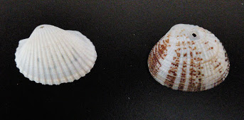
We will be measuring several variables on two different kinds of clam
shells - white (left) and calico (right). Although both of these are
bivalve shells, and have a roughly similar morphology, we will use
multivariate techniques to see how they differ across several
morphological measurements at once.
Everyone should measure 2 or 3 shells of each type until all are
measured. Make sure you measure each variable on the shells you select -
one missing variable forces us to drop the entire shell from the data
set! Please measure carefully.
The measurements we will use will be:
Weight - weigh the shells on the
balance.

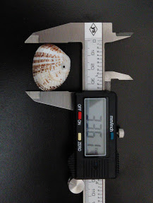
Major axis - maximum distance measured along the
longest dimension, with a calipers, to the nearest 0.01 mm.

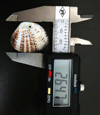
Minor axis - maximum distance measured roughly
perpendicular to the major axis. Make sure the shell sits flat along the
jaws of the calipers.

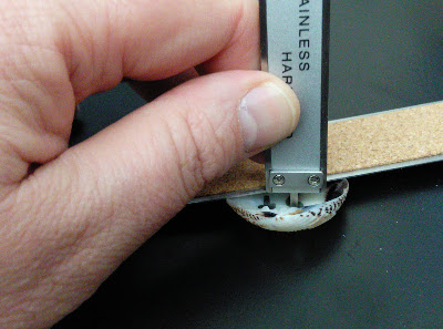
Height - measured from top to bottom. Be careful that
both sides of the open part of the shell rest on the jaws of the
calipers, and not in the gap at the back.

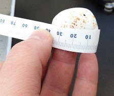
Surface length - use a tape measure to to measure the
surface distance along the major axis. Record this to the nearest 0.5 mm
(between the 1 mm hash marks).


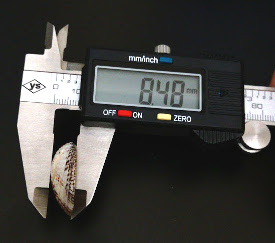
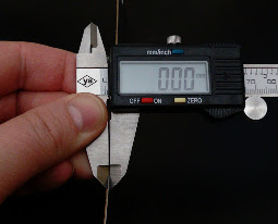
Depth - measure the thickness of a metal ruler and
zero the calipers on it. Then, lay the shell on the ruler, and measure
the depth from the top of the ruler to the inside of the shell at its
deepest point using the bottom of the caliper as a depth gauge.
Each of you should measure 2 or 3 shells of each
kind, until all are measured. Enter your data in the shell data form
linked below these instructions on Canvas.
Buffalo incisor morphology

Hoofed mammals with even numbers of toes are placed in the Order
Artiodactyla, and Artiodactyls with permanent horns are placed in the
Family Bovidae. Bovids are predominantly grazers (i.e. they eat grass),
and their teeth are adapted to this diet. Their cheek teeth (i.e. molars
and pre-molars) are adapted for grinding up grass. We won't be working
with cheek teeth today.
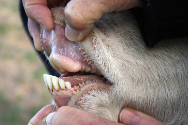
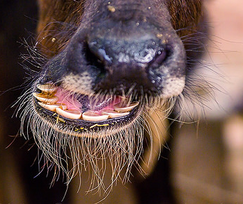
Bovids have incisors that they use to clip off grass to eat, but only
on their lower jaw (as you can see in the first picture with both the
upper and lower jaw visible). They press the grass against a thick,
tough dental pad on their upper jaw, and then clip off the grass against
their incisors.

We have 100 teeth from an Indian buffalo species, like the one shown in
these pictures. The incisors are expected to vary in size for a couple
of reasons: a) individual variation, and b) variation attributable to
position in the mouth. As you can see in these two pictures, the teeth
in the middle at the front of the mouth are bigger than the ones towards
the back of the mouth. The pictures also suggest we will see variation
in shape, as the tooth shape also appears to change with position.
Teeth are complex objects, and we will discuss as a
class what variables we should use to characterize variation in size and
shape.
Each of you should measure 3 or 4 teeth,
until all are measured. Enter the data in the form on Canvas, below the
link to these instructions.
LandSat reflectances by cover type

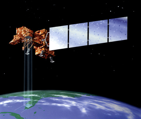
NASA and the US Geological Survey jointly operate the LandSat remote
sensing program, which uses satellites to record reflectance of
electromagnetic radiation from the earth's surface. At least one
satellite has been in orbit continuously since 1972, and the orbital
paths allow each satellite to record the same location about once per
month. We will be using an image from the LandSat 5 satellite taken in
April of 2011 that covers most of San Diego County.
If you are familiar with how a digital camera works, visible light is
recorded in three different bands (red, green, and blue), and these
three primary colors of light are combined on the page, or on a computer
screen, to make all the colors we see. Digital images are an array of
square pixels, each of which have a digital
number recorded that indicates the amount of light that was
recorded in the band. Digital numbers can have values between 0 to 255,
with 0 indicating no light recorded in that band, and 255 being the
maximum amount of light that the sensor can record in that band.
For a typical color image, a single pixel on the screen will thus have
a DN for each of the three recorded color bands, reported as an RGB
code. For example, an RGB code of 255,0,0 would have a maximum amount of
red, and no green or blue, which will display as bright red on the
screen. An RGB value of 255,255,255 is white, an RBG of 0,0,0 is black,
and any set of numbers that are the same is a shade of gray (150,150,150
would be a medium gray, 250,250,250 would be a very light gray).
LandSat satellites record all three of the visible light bands, but
they also include additional bands that are not visible to the naked
eye. The LandSat 5 sensor that recorded the image we will use had 7
bands, the first three of which were visible blue, green, and red, and
the remaining four of which were infrared (band 4 and 5 are near
infrared, band 6 is mid infrared, and band
7 is thermal infrared).

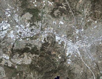
The LandSat data can be used to make color composites that either look
natural (if they use only the three visible bands), or that don't look
natural (if one or more of the infrared bands is assigned to the R, G,
or B channel on the computer monitor). Assigning the bands that record
visible red, visible green, and visible blue light to the R,G, and B
channels on the computer monitor gives you a "true color" composite,
like the one on the right. You can see that different types of land
cover have different colors - this is because different cover types
absorb more light in some bands and reflect more in others, which gives
us a different mix of R, G, and B digital numbers for different cover
types.

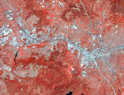
But, we have more than the three visible bands to work with. If we
assign the first near-infrared band (band 4) to the red color channel on
the computer screen, we get a "color infrared" image. Visible blue and
visible green are still assigned to the blue and green channels,
respectively, but just by substituting infrared for red we can see
certain differences more clearly than before, and we can also see some
differences in the vegetation that wasn't apparent. It turns out that
actively growing vegetation reflects more strongly in the infrared bands
than does living but less active vegetation, and even more strongly than
does dormant or dead vegetation.
The problem to solve - no cover type information is
recorded
Now, although the color variation is obviously due to differences in land
cover, the computer doesn't know this yet. If we clicked on a point on the
map we could retrieve the DN's for all seven LandSat bands recorded for a
pixel, but we couldn't get the cover type for that pixel because that
information hasn't been assigned to the pixels.

What we can do, though, is extract all seven DN's from a sample of the
pixels taken within areas of known cover type and use that information to
test whether there is a collection of DN's that's distinct for each cover
type (a spectral signature, as it's called). If the
spectral signatures are different for the cover types we're interested in,
we could then classify the cover types for all the pixels in the map by
matching the spectral signatures of the unknown pixels to the spectral
signatures of the known pixels.
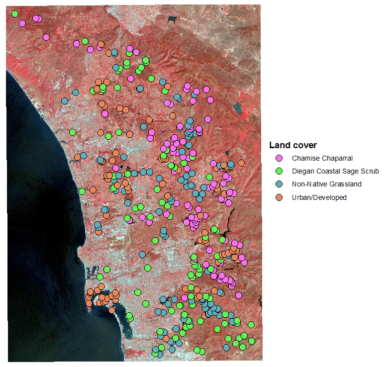
I randomly generated 400 points in areas that had one of five known cover
types (100 in each cover type), shown to the right.
To collect the data, one of you will need to "extract" the digital
numbers from the seven bands into the attribute table for the points.
The data sets are on the P: drive, in folder
P:\Biology\wkristan\biol532\landsat. You may need to make a folder
connection to P: to access the files.
1. The rand_points.shp attribute table will be changed during this
analysis, so you will need to put a copy of it in a folder you
can write to on your H: drive. You can use ArcCatalog to copy
the file from P: and paste it to a folder on your H: drive.
2. Load the data into ArcMap. Use landsat_april11.img from the P: drive,
and the copy of random_points.shp you put on your H: drive.
3. Open ArcToolbox, and launch "Spatial Analyst Tools" → "Extract Multi
Values to Points".
The "Input point features" is rand_points.shp, and the "Input rasters" is
landsat_april11.img. Click "OK" to run.
That's it - call me over and I'll show you which file to upload to the
course web site.
