 ,
Bald eagle
,
Bald eagle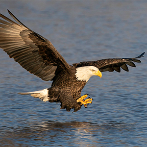 ,
Northern Harrier
,
Northern Harrier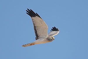 ,
Red-shouldered Hawk
,
Red-shouldered Hawk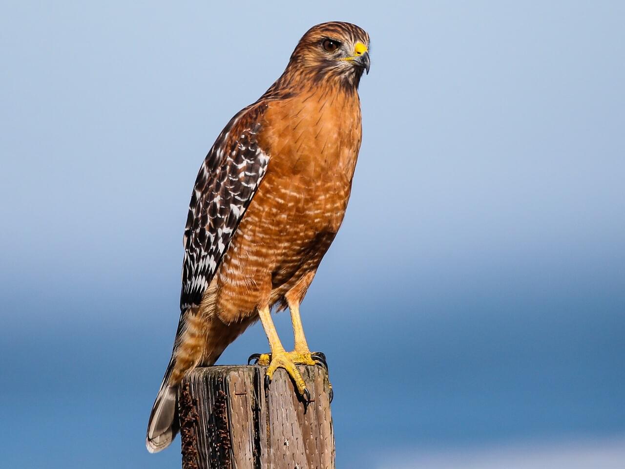 ,
and Merlin
,
and Merlin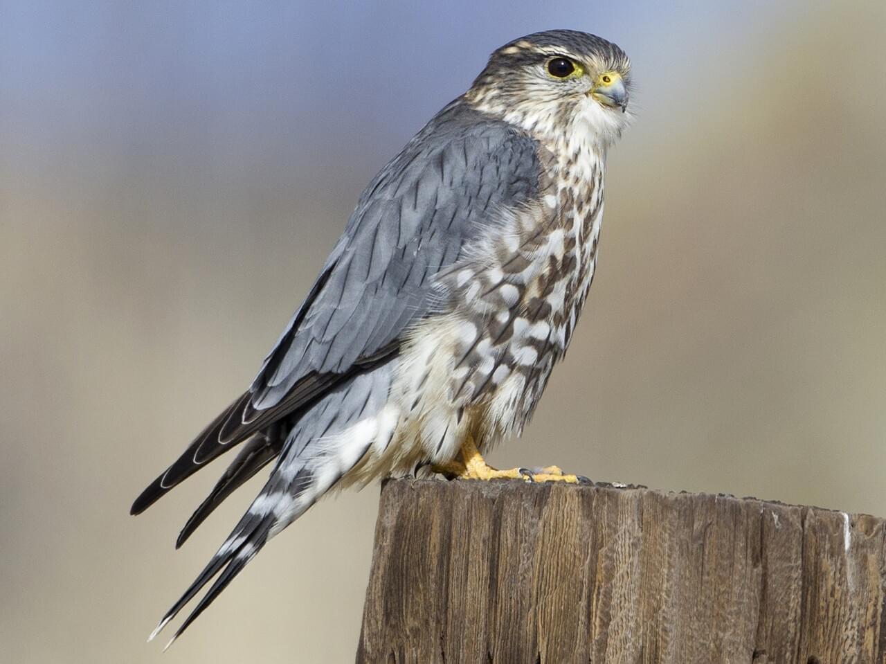 .
.We will be looking at trends in counts of a set of birds of prey, using two different monitoring programs: the Breeding Bird Survey (BBS), and Hawk Mountain's annual migrating hawk counts.
Both data sets we will work with are relatively long-term. BBS began in 1966, and focuses on counts of birds during the breeding season. BBS data are collected from throughout North America, but with densities of routes being related to human population density. The Hawk Mountain data records raptors during their Fall migration, and the counts are done from a single location. However, since the Appalachian Flyway, a major travel route for migrating birds along the East Coast, goes right over Hawk Mountain, PA, raptors from all over eastern North America pass by that one location. Counts have been done at HM annually since 1934, every year except for 1942-1944, when they took a break to fight World War II. There are thus a total of 74 counts conducted over 76 years.
Raptors are carnivores, and as such were one of the groups of birds most strongly affected by DDT, an insecticide used from the World War II era through its eventual banning in the US in 1972 (although it was not banned worldwide until 2001). DDT is a persistent, fat-soluble chemical that enters the food chain, and bio-magnifies, meaning that its concentration increases as it moves up to higher trophic levels. Top predators thus would have massively higher concentrations in their tissues than the concentration applied in the environment. DDT was thought to be non-toxic to vertebrates, but it was found that at this very high concentrations it leads to eggshell thinning and reproductive failure in birds. Several species, including the Bald Eagle, ended up listed as Endangered Species primarily due to DDT.
BBS data can be downloaded for analysis, but there are statistical issues that need to be accounted for that go beyond what we will be addressing in this class. However, the USGS Patuxent Wildlife Research Center has developed a web-based analysis platform that we can make use of.
Our goal for today, then, is to use the BBS web site to analyze trends in a selection of raptors in eastern North America, and then conduct our own analysis of Hawk Mountain data on the same species. We will see whether counts of breeding and migrating birds tend to tell us the same thing, or whether they indicate different trends in these species.
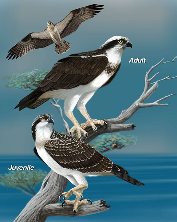
The species we will use are Osprey,
Bald eagle,
Northern Harrier,
Red-shouldered Hawk,
and Merlin.
We will keep this section short and sweet - follow this link to the Breeding Bird Survey's regional trend analysis page. Scroll down to the "Survey Results" section, and then select "Trend Estimates" that are conducted by species.
Download this file to your S: drive, and open it in Excel. You'll see that it's an Excel spreadsheet with one worksheet called "BBS", followed by a different worksheet for each species with data from the Hawk Mountain counts, and one final one for import into R - we'll get to those next, first switch to the BBS worksheet.
Find the first species, Osprey, in the drop-down menu of species (they are listed in a taxonomic order instead of alphabetically, so you may have to search around a little). You'll see that there are two trends listed for each area: one for the entire BBS period (1966 to 2015) and one for the most recent 22 years of data (1993-2015). Find the Eastern BBS Region (near the bottom of the list), and record the trend estimate, the lower limit and upper limit for confidence interval in your worksheet (you don't need to record the RA score, this is a measure of relative abundance of the species relative to other species in the area, which isn't relevant to us).
For the 1993-2015 estimate, enter whether the trend estimate indicates an increasing population, a decreasing population, or a stable population (column E). The trend estimates are changes in number of birds counted per year, and the confidence interval will tell you whether you can consider the trend to be different from zero; if the confidence interval includes zero, consider the population stable. If the confidence interval does not include zero, and the trend estimate is positive, then it's an increasing population. If the confidence interval does not include zero, and the trend estimate is negative, then it's a decreasing population.
Repeat the increase, decrease, or stable designation for the 1993-2015 estimates (in column I).
Now, compare the two conclusions in E and I for each species: If the two trend estimates lead to the same conclusion, then enter "no change" in J. If there was a shift either from decrease to stable or increase, or from stable to increase, then things have been improving lately - enter "Accelerating" in column J. If there is a shift from increasing to stable or decreasing, or from stable to decreasing, then things have gotten worse lately - enter "Decelerating" in column J.
Repeat this set of steps for the other four species: Bald Eagle, Northern Harrier, Red-shouldered Hawk, and Merlin.
Once the BBS numbers are entered in your Excel file you can move on to analyze the Hawk Mountain migrating raptor data set, and see how it compares to what we see in the BBS counts.
We will be analyzing the changes in number of migrating birds counted at Hawk Mountain next. The data are collected from an observation point at the top of a mountain, and the species is recorded for each bird observed. The data were tallied by day between 1934 and 1965, and by hour thereafter. The number of days and hours were variable, but the number of minutes of observation was recorded for each observation period, so I was able to calculate the number seen per minute, multiply that by 60 to obtain a number seen per hour, and then average these numbers per hour for each year. The data we will work with, then, is the mean number of birds of each species observed per hour of observation for each year.
With such a long time series we will have the opportunity to see many trends that are not simple linear relationships. If you think about it, linear relationships can't be common in the long term - species may decline linearly for awhile, but will eventually go extinct if they don't level off. Species may increase linearly for awhile as well, but they will eventually deplete their food source and either stabilize or crash to smaller numbers. We will be using non-linear regression to describe the changes in numbers over time for each of our species.
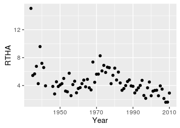 |
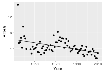
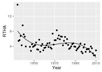
Consider the data to the left for the Red Tailed Hawk. We're interested in whether they are stable, increasing, or decreasing over time, and linear regression will give us a slope coefficient that will address that. So let's see what a simple linear regression looks like. |
 |
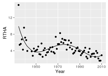
Based on this linear regression there does seem to be a decline in RTHA over time, but notice that the line doesn't fit the data very well. There is a marked decline to about 1950, with an increase after about 1960, to a peak at about 1975, with a decline after that. A straight line with a single slope is simple and easy to interpret, but if it doesn't describe the data well we shouldn't try to interpret it. Think of a straight line is a first-order polynomial - a slope multiplied by x raised to the power of 1, RTHA = b + m(year1). The next highest would be a second-order polynomial, which is also called a quadratic function, so let's try fitting a second-order polynomial to these data. |
 |
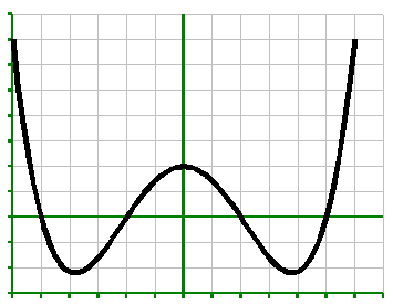
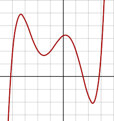
Adding a polynomial gives the regression the ability to follow a pattern that is predicted by the polynomial. You'll see in the example on the right of three different parabolas that they can point upward or downward depending on the sign on the coefficient, and small coefficients make them flatter. The linear term has to be kept in the model, but when we add a quadratic (i.e. squared, parabolic) term we can describe patterns that have an n or u shape. This graph may look the same as the straight line above, but it's not. The formula for this line is RTHA = b + m1(year1) + m2(year2), but the pattern is not at all a parabolic curve, so the coefficient on the year2 term, m2, is nearly zero.
|
 |
 |
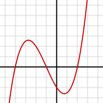
Cubic functions are like a sideways s-curve - they can rise, fall, and then rise or if we flip them around the x-axis they can fall, rise, and then fall (click on the graph to flip it around the x-axis). If we just used the middle portion we can have a forward or backward s-curve with a cubic term included (click to see the s-curve created from the middle section). The cubic added to the formula gives us the graph to the left, and the formula is: RTHA = b + m1(year1) + m2(year2) + m3(year3) This is looking better - we've captured the general shape, but are under-shooting the increase in the 1970's, and perhaps over-estimating the recent decline. |
 |
 |
A fourth-order polynomial looks like the graph on the right - click to flip it around the x-axis. Fitting a fourth-order polynomial to our data, with the formula: RTHA = b + m1(year1) + m2(year2) + m3(year3) + m4(year4) gives us the graph to the left. This too is closer to the data, but the uptick at the very end is a little optimistic - we're still under-shooting the increase in the 70's a little as well. |
 |
 |
Finally, a fifth order polynomial looks like the one on the right. Using the formula: RTHA = b + m1(year1) + m2(year2) + m3(year3) + m4(year4) + m5(year5) gives us the graph on the left. This is a very good description of the data - still under-shooting a little in the 1970's, but the line is going through the data well in the last couple of decades without an artificial upturn in the last few years. |
 |
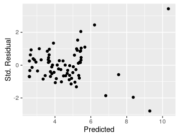 |
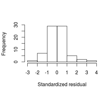
How do we know this is the right relationship to use? We can look at a couple of things. First, the fact that the line (mostly) goes through the middle of the data is a good sign that this is a good description of the data. We can augment this impression with plots of residuals, like the residual vs. predicted plot on the left, and the histogram of residuals on the right. |
 |
The other thing we can do is to compare the different models against each other to see whether we are doing a better job of characterizing the data by adding higher order terms - this type of comparison is done by comparing the unexplained variation in two models. This type of comparison is only statistically valid if one of the models is a subset of the other. If you look at the formulas for the fifth and fourth-order models, the fourth only has terms that are in the fifth, but the fifth has just one extra. That means the fourth order model is a subset of (or "nested" within) the fifth. If we compare them we would find that we don't have significantly more variation explained by the model with the fifth order term (p = 0.3591).
But, look at the graphs above - the fourth-order model has a dramatic up-swing in the last few years of the data, but the data doesn't show such a pattern. The line is the "best fit" fourth order polynomial across the entire data set, but it's not fitting well in the last few years, which (from a management perspective) are very important. This is one of the downsides of using polynomial regression - the function imposes a shape to the line that may not be well supported by the data, so it's important to make sure the line fits the data well. We may choose to stick with the fifth-order model because of its better fit in the last decade or so of the data set. This is a very high-order polynomial to use, by the way - beyond about 4th or 5th order the equations become very complex, but usually high-order polynomials don't dramatically improve the fit of the model to the data. At the extreme, with 74 years of data we could fit a line that hit every single data point perfectly with a 73rd-order polynomial, but it would be useless for understanding the general trend in a mean number of birds over time, with random variation around it.
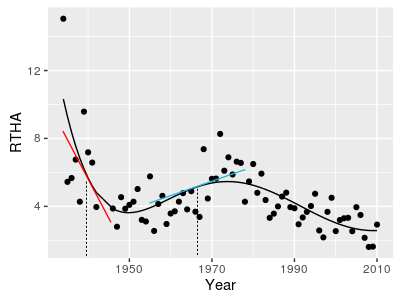 |
Once we have a line that fits the data well, we can use it to address how RTHA have changed over time. With a complex pattern of change like we're seeing for RTHA there isn't a single rate of change that describes the data. We do get coefficients for each of the terms in the model, but they are constants, and don't tell us what is happening at any given year. Instead, the rate of change at any year is a tangent line to the curve at that year. For example, in 1940 the tangent line (in red) has a strongly negative slope, but by 1967 (in blue) it's moderately positive. We can calculate the slopes of these tangent lines at any year of interest using the first derivative of the function. |
With polynomials, derivatives are easy to calculate - you drop the constant (b), and multiply the coefficients (m's) by the exponents, and then subtract 1 from the exponents.
So, with our fifth-order polynomial, the equation was:
RTHA = b + m1(year1) + m2(year2) + m3(year3) + m4(year4) + m5(year5)
And the first derivative with respect to year, d(RTHA)/d(Year), is:
m1 + 2m2(year1) + 3m3(year2) + 4m4(year3) + 5m5(year4)
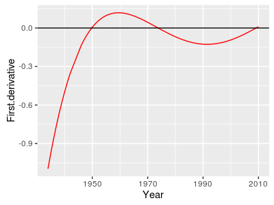 |
A graph of the first derivative is shown to the left. The horizontal black line at 0 indicates a stable population - neither increasing or decreasing. In years that the first derivative is positive (above 0) Red-Tailed Hawk counts are increasing. When it's negative, the counts are decreasing. |
Okay, now with that background, let's analyze some hawk data.
1. Plot the first species change over time. Switch to the first sheet of Hawk Mountain data, Osprey. You'll see that Year is expressed in two ways, as the calendar year (from 1934 to 2010) and as the "year.number" from 0 to 76. Year.number is just the number of years since the beginning, and is obtained by subtracting 1934 from each Year. We need to do this to make it possible to estimate the higher-order terms (to work with a fifth-order term you have to raise year to the fifth power, and if we raise 2010 to the fifth power we get numbers that Excel can't handle).
Select the data for Year.number and OSPR, including the column headings (B2 through C75), and insert a scatter plot:
Make sure it's a scatter plot, and not a line plot with just plot symbols - line plots treat the x-axis as categories, even if the x-axis variable is made up of numbers, and we need the x-axis to be numeric or our polynomial regression lines won't be accurate.
The axes are not labeled by default, so let's fix that - click on the x-axis labels and you'll see three tools pop up to the right - click on the + tool to add axis labels, like so:
Change the x-axis label to "Year number" and the y-axis label to "Sightings per hour".
2. Add trend lines. Select the data by clicking once on the dots. Click on the + (Chart Elements) and select "Trendline" → "Linear", which will add a linear regression line to the graph.
You'll see it doesn't fit very well, as there seems to be an increase in osprey in the first several decades, but then the numbers level off in the 1980's, around year 45. Because of this the "best fit" line over-shoots in the early and later part of the series, and under-shoots in the middle years.
Next, to get the R-squared and regression equation onto the graph, select the trend line, and then in the settings panel on the right side of the spreadsheet, find the boxes for "Display Equation on chart" and "Display R-squared value on chart", and check the boxes next to each of them. You can move the box with the equation and R2 to a location you can see them, like so:
Note that I made my line thick, red, and solid to make it easier to see, yours may be blue and dotted instead. R2 is useful to us because it is the proportion of the total SS that is explained by the line - we'll use this later when we compare the lines against each other in the next steps.
We can add a polynomial line next - this time, select the dots on the graph, right-click and add a trendline. This will give you a second line, but it's sitting right on top of the first. In the "Format Trendline" window that opens up you can select a "Polynomial" trend line, and set it to order 2 - this will be a model like the one above for RTHA that has both the linear and quadratic terms. Also have the R-squared reported on the chart, and move them where you can see them - they aren't labeled as "quadratic", but you can see that the equation is -0.0002x2 + 0.017x + 0.1896, and the fact that there is a squared term in the equation tells you this is for the quadratic trend line.
Switch to the "Fill and Line" settings in the "Format Trendline" window, and change the line color to something that's different from the straight line, and easy to see.
Now, back to the "Trendline options" where you started - you can try out polynomials of different order by increasing the number on your quadratic fit. Try 3, 4, and 5. You'll see that going to 3 changes the shape a little - it flattens out the early part of the curve and makes it peak more sharply in the late 1990's. After that increasing the order of the polynomial barely changes the shape of the line - this is a pretty good indication that these higher-order terms aren't helping to describe the pattern of change.
Next we will learn how to test whether adding a term significantly improves the fit of the line to the data.
3. Test for an increase in fit as you add higher-order terms. We are going to build a table that tests whether the quadratic fits better than the linear, whether the cubic fits better than the quadratic, whether the fourth order fits better than the cubic, and whether the fifth order polynomial fits better than the fourth order.
The basic idea is that we need to know how much additional variation we are able to account for in the count data by adding each higher-order term. If the amount is large enough to be statistically significant, we have justification for including the term. When we get to a point that adding higher-order terms no longer improves the fit, we can stop and interpret the simplest model that fits the data well.
Remember from the regression review, we can divide the sums of squares for the bird counts into a portion that can be explained by a line through the data (the model SS), and a portion that is random, unexplained variation (the residual SS). As we go from a straight line to a quadratic model, the quadratic will fit the data better by some degree - we can calculate the difference in the unexplained, random variation as a measure of how much additional variation is explained. We can use this additional explained variation in an F test, in which we divide the MS for the explained variation by the residual MS. This is very much like the F-test we conduced in the ANOVA table we produced for our simple linear regressions, but in this case we're testing for significant increases in fit by making the model more complex.
Now to calculate the values for the table.
Your table should look like this:
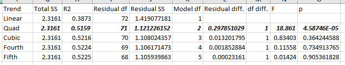
Based on these calculations, we significantly increased the explained variation when we added the quad term, but not when we added the cubic term, the fourth-order, or fifth-order terms. Consequently, we'll base our interpretations on the quadratic model.
Select everything in the Quad line, and hit CTRL+I, then CTRL+B to italicize and bold the characters for the model you will be interpreting.
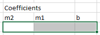
4. Calculate the coefficients for the first derivative. Now we want to know what the change in Osprey count per year is, at any given year. We need to calculate the first derivative of the quadratic to do this - it sounds hard, but it's actually not.
5. Calculate the rate of change each year. You may already know that the first derivative of a parabola is a straight line, and sure enough we now have a constant and a slope to multiply by year for our first derivative, which makes it a straight line.
In cell D1 type "Rate of change", and in cell D2 type =g$14+f$14*b2. Copy and paste this to the rest of the years. If you look down the Rate of Change column you'll see that the rate of change was positive until about 1990, when Osprey started declining.
6. Plot the rates of change. Select Year.number and the rates of change, and insert a scatter plot with only connecting lines and no plot symbols. These columns are not sitting right next to each other, but you can select the Year.numbers first (by clicking on B1, holding, and dragging to the bottom of the year numbers in cell B75), and then holding down the CTRL key and clicking, holding, and dragging on the Rate of Change values in column D.
To get the scatter plot with lines and no plot symbols, click on the scatterplot icon in the Insert tab again,
but this time select the option that shows only straight lines with no symbols, 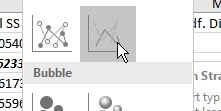 .
.
You can add a title, and title it "Rates of change in Osprey counts". The axis labels are still "Year number" for x, and "Change in osprey number" for y.
7. Repeat. Now you can repeat this for the other four species. Specifically, for each species:
A couple of hints...
When you're done, make sure you can interpret the rates of change graph - which years show increases, which show decreases, and in which were they stable?
Also look at how the trends compare for breeding birds and migrating birds - year 32 is 1966, and year 76 is 2010, so are the rates of change you're seeing for those time periods in agreement with the BBS trends? Note that the units are different on the BBS data - they are numbers of individual seen per route surveyed. When comparing between BBS and Hawk Mountain trends focus on the sign on the trend, and whether the trends were different for recent counts than overall for each species.
Download this Rmd file to the same folder the hawks.xlsx file is in, start R Studio, and make a new project from an existing folder using the folder with the data and Rmd file in it. Open the Rmd file and follow the instructions. For this kind of statistical analysis you'll see R is actually much quicker and easier to use (you have to know a little more about what you're doing to make the graphs work, but comparing the model fits is much easier). Do the Osprey trend analysis, and then feel free to do other species if you want the practice.