Likelihood methods have been a boon to ecologists - they make it possible to estimate all sorts of population
parameters that we're interested in, from population size to survival probability. Likelihood makes it possible to
not only get estimates of parameters from models fitted to data, it allows us to compare how well different models
are supported by the data so that we can pick the best model on which to base our conclusions. We can also obtain
valid confidence intervals for estimates using the same likelihood function we use to find the estimates
themselves - obtaining confidence intervals that won't go above 1 or below 0 for estimates of proportions turns
out to be a surprisingly hard problem to solve without likelihood. Likelihood is all over the ecological
literature, but it may still be unfamiliar to you, unless you have already taken an advanced statistics class like
Biol 531.
We will start using likelihood in the next lab to estimate population size, but before we begin to rely on it to
make sense of data we will get a little practice with it today by reproducing the maximum likelihood estimation of
the binomial coefficient, p, that I showed you in lecture.
Remember,
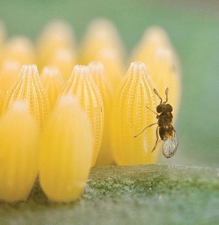
the data are numbers of times that a parasitoid wasp selected a mated butterfly to hitch a ride on - since the
wasps lay their eggs on the butterfly's eggs, selecting a butterfly that has bred increases the wasp's chances
that the butterfly will soon lay eggs, and increases the wasp's chances of successfully reproducing. The question
is, can the wasps tell the difference between a mated and a virgin butterfly, or are the wasps just hopping on the
nearest female butterfly and hoping for the best? The experiment I showed you simultaneously presented a female Trichogramma
wasp with a choice of a virgin butterfly and a butterfly that had already mated, and recorded which butterfly the
wasp selected. If the wasps were selecting at random, they should have selected mated butterflies 1/2 of the time.
The researchers conducted 32 trials, so if the wasps were guessing 32/2 = 16 times they should select mated
butterflies.
Out of a total number of trials of 32, 23 times the Trichogramma females selected a mated butterfly -
not all the time, but more than the 16 times expected if the wasps were guessing.
We would like to use these data to estimate the probability that a wasp will choose a mated butterfly in any
single trial, and we have been told by those who supposedly know better that proportions of totals can be used as
estimates of probabilities - so, we could estimate the probability that a female wasp will choose a mated
butterfly as p = 23/32 = 0.71875.
But, this leaves us with some questions:
How do we know that this is the best estimate of p?
Since the experimental outcome is subject to random variation, 23/32 is only a point estimate of p (we can
call it p̂ to make it clear we are talking about an estimate). If it is only an estimate, we should also have a
confidence interval that tells us how good an estimate it is, so what is the 95% confidence interval for this
value?
The first question we will answer by confirming that 0.71875 is the maximum likelihood estimate
for p. By definition, the maximum likelihood estimate for a population parameter is the value most likely to have
produced the observed data. If you recall from our regression review, the least squares criterion
was used to identify the best fit line - that is, the line that minimized the squared residuals was the best fit
line. The maximum likelihood criterion serves the same purpose here, in that it gives us a way
to evaluate which of the infinite possible values for p is the best one. And, if you're curious, the least squares
line is also the maximum likelihood line if the residuals are normally distributed (this is one of the reasons
that we test for normality of our residuals in a regression).
The second question is actually a hard one to solve. It's possible to use the Wald method to
calculate a 95% confidence interval for a proportion - this is the same method we used for calculating a 95% CI
for the mean; namely, we calculate a standard error for the proportion, and then add and subtract as many of them
as is needed to capture 95% of the possible values for p. The problem with that approach is that the interval
would be symmetrical around p̂, but p can't be lower than 0 or higher than 1. As p gets anywhere near those
basement or ceiling values, adding and subtracting a fixed uncertainty level from the mean can put the upper limit
above 1 or the lower limit below 0; a confidence interval that tells us that impossible things are possible is not
very useful. Using maximum likelihood we can calculate 95% confidence intervals that are asymmetrical around the
estimate of p, and that can't go over 1 or under 0.
To understand the problem to be solved, look at the graph below.
Value of p̂:
Sample size:
If you either reduce the sample size, or move p̂ to larger or smaller values you'll see that
the interval crosses over into negative numbers or numbers greater than 1, neither of which are possible
proportions.
The Wald method work better as the sample size increases - if you increase the sample size while the value of p̂
is kept at either 0.4 or 0.6 you'll see that the Wald interval gets smaller, and contracts out of impossible
values. The color of the interval is red when it includes impossible values and black when it does not (it has to
be symmetrical because Wald intervals add and subtract the same uncertainty value, so the upper and lower limits
will always be the same distance from the estimate). Large sample sizes solve all kinds of statistical problems,
but when we have smaller sample sizes we have to be careful in our choices.
Likelihood will give us a better method for dealing with this problem that still works even when sample sizes are
small.
Maximum likelihood estimation of a proportion
As we move on to likelihood-based estimates of population size and survival probability we will be working with
likelihood functions that can't be solved for parameters that we want to estimate, and we will have to use trial
and error approaches (called numerical solutions) to get our estimates. We will use an Excel
extension called the Solver to get exact numerical solutions in the next lab. To help you understand better how
likelihood works we will work with a set of evenly spaced values of p, with likelihood calculated for each one, so
you can more easily see how maximum likelihood estimation works.
1.Lay out values of p to be possible estimates. Use the same file that you used last time to
estimate population size using the Lincoln-Peterson estimator - switch to sheet "Binomial", which is blank, and
you will do all your calculations there.
Enter "p" into cell A1. In cell A2 enter 0.5. In cell A3 enter 0.51. Like so:
Now, select both A2 and A3, and use that fill handle you're so fond of to extend the sequence up to 0.99 (it will
end in cell A51). These are the estimates of p that we will try out.
2. Calculate the likelihood function for each value of p̂. Enter the
observed data into the sheet - enter the label "Mated" in H1, "Virgin" in H2, and the numbers 23 and 9 in i1 and
i2, respectively.
In cell B1 type "Binomial". We will use the binomdist() function to calculate the probability
of getting 23 out of 32 mated butterflies when the probability of selecting a butterfly in each trial is equal to
the values in column A. These probabilities can also be interpreted as likelihoods of the value of p̂ given 23 of
32 mated butterflies were selected.
In cell B2 type =binomdist(i$1, i$1+i$2, a2, 0)
When you hit ENTER you will see a value of 0.0065, which is the probability of getting 23 mated butterflies (from
i$1) out of 32 trials (the sum of i$1 and i$2) if the probability a wasp will select a mated butterfly is 0.5 (the
value in A2). The final argument, by the way, specifies whether we want cumulative probabilities - setting this to
0 gives the probability of exactly 23 out of 32, not the sum of all of the outcomes from 0 to 23 out of 32.
Remember, likelihood is different from probability, but we use probability distributions for likelihood
functions - the difference is in the interpretation, not the calculation. The way to interpret this number as a
likelihood, then, is that the likelihood that p = 0.5 given that we got 23 out of 32 mated butterflies is 0.00653.
What does this mean? Not a lot by itself, we need to compare it to other estimates of p.
So, to get
some other values copy and paste cell B2 to the rest of the cells (B3 to B51). You can either copy and paste B2 to
the rest of the rows, or use the fill handle. When you have a set of values already entered, double-clicking on
the fill handle extends extends the cell down to the bottom of the cells next to it, like in the animation to the
left. Since the number of mated and virgin butterflies was entered with dollar signs for their row numbers their
cell references will not change as you copy and paste to rows below, but the formulas will update to point to each
new estimate for p̂.
3. Find and highlight the maximum likelihood estimate. Now that you have likelihoods for 50
candidate values of p, find the best one - scan through the values and see which is largest. When you find it,
make it bold italics. We're rounding to the nearest 0.01, but you'll see the value 0.71875 rounded is 0.72, which
is the estimate with the largest likelihood of the 50 we are considering. So far so good.
4. Consider the likelihood function. Let's look at what you're doing with a couple of graphs.
Below, the graph on the left shows the number of virgin and mated butterflies, and the graph on the right shows
the likelihood function for our estimates of p. A good way to think about what a proportion represents about the
data is that it is the balancing point - if you think of the graph as being a teeter-totter with 9 blocks stacked
on the left and 23 on the right, p is where you need to place the pivot point to get the teeter totter to balance.
The graph on the left is set up to tilt when p is away from the balancing point - move it too far to the left
(i.e. too small an estimate) and the tall stack on the right causes it to tilt in that direction. Move the pivot
point too far to the right (i.e. too big an estimate) and the weight of the bar on the left gets too far away and
tilts the teeter totter in that direction. At the initial value of p̂, which is set to 0.5, we are too far to the
left, and the graph is tilted right. The likelihood for the current value of p is shown as a red dot on the
likelihood function - not surprisingly, the value 0.5 has a low likelihood given the data.
As you move the slider to find the best value of p, you'll see that the red dot reaches the peak of the
likelihood function when p̂ is equal to 0.72 - at this point the graph on the left also balances and becomes flat.
Switching from likelihood to log-likelihood (by dropping down the menu below the slider and selecting it) changes
the shape of the curve but doesn't change the location of the maximum - the same value of 0.72 maximizes the
log-likelihood. Switching again to the negative log-likelihood flips the curve upside down, so that we now find
the value of p̂ that minimizes the negative log-likelihood, but the location of the minimum is the same as the
location of the maximum of the other two curves.
If you change the number of mated butterflies from 23 to a higher or lower number the curve changes, but the
value of p̂ that maximizes the likelihood will always be equal to the number of mated butterflies divided by the
total number of trials. This shows us that dividing a part by the total is a maximum likelihood estimator for p.
Number mated:
out of 32 trials
5. DIY likelihood - drop the unneeded counting part. We can use probability distributions as
likelihoods, but probability distributions contain terms that ensure that the area under the curve is equal to 1,
and we don't always need them - we can often simplify the likelihood function by dropping them without changing
the estimate. For example, the binomial distribution's equation is:
We are estimating p, but p doesn't appear in the "counting part" (the part that tells us how many different ways
there are to get 23 mated out of 32 trials), so we can drop it from our likelihood, leaving us just with:
Without the counting part this is no longer usable as a probability distribution, but it is still a perfectly
good likelihood function. We can calculate this version of the binomial likelihood function ourselves with a
spreadsheet formual - in cell C1 type "NoCount", and in cell C2 type:
=(a2^i$1)*((1-a2)^i$2)
This gives you the likelihood of p = 0.5 given 23 mated and 9 virgin butterflies. If all went well it will be
equal to 2.32831E-10.
Copy and paste the cell to the rest of the cells in the column, and check that this calculation also maximizes at
the same value of p̂ - this is a demonstration that using the version of the likelihood function without the
counting part gives us the same estimate for p (bold and italicize it).
6. Calculate the log likelihood. We now want to work with logs of these likelihoods so that we
can start working on the 95% confidence interval for our ML estimate. In cell D1 type "LnLikelihood". We could do
this calculation in a couple of different ways....
Since you already have the likelihoods in column C, you could type =ln(c2) into cell D2 to get your log
likelihood (the function ln() is the natural log, or the log to the base e = 2.718). Go ahead and do this, and
note the value - it's -22.1807 (remember, logs are the exponent needed to raise a base to get a
number, and since the likelihood is a decimal number the natural log is negative).
The other way to do the calculation is to take the log of the likelihood function - the log of pr(1-p)(n-r)
is:
r ln(p) + (n-r) ln(1-p)
We can do this calculation to confirm it's the same as ln(c2) - in cell D2 change the formula to:
=i$1*ln(a2) + i$2 * ln(1-a2)
You should still see a value of -22.1807. Copy and paste this to the rest of the cells. Check that the ML
estimate is still the same - the log of the likelihood function should still maximize at the same estimate (don't
forget that negative numbers are considered bigger if they are closer to 0, so the negative number with the
smallest absolute value is the largest number).
7. Calculate the negative log likelihood, and make it touch the x-axis at the minimum. Now we
will calculate the difference from the maximum likelihood. To get our 95% CI, we will be looking for the
likelihoods that are within 1.92 units of the maximum. To make this easy to find, type "Difference from max." into
cell E1. In cell E2 type:
=max(d$2:d$51) - d2
This will give you the difference between the log-likelihood for p = 0.5 and the maximum log-likelihood, for p =
0.72. Copy and paste this to the rest of the cells - it will be 0 for p = 0.72, close to 0 for values of p close
to 0.72, and increasingly large as you move towards 0.5 or 0.99.
Note that doing the differencing in this direction gave use the negative log likelihood. The
values are positive, and the p̂ at the minimum of the negative log likelihood is also the p̂ at the maximum
of the log likelihood. The difference between the maximum and itself is 0, so we made the curve touch the x-axis
right at the maximum likelihood estimate.
8. Find the lower and upper CI bounds. The negative log-likelihood follows a Chi-square
probability distribution, which we can use to find the confidence interval limits. The critical value for
Chi-square with a confidence level of 0.95 is 3.84 - to divide the probability between the upper and lower tails
we divide this in two, which gives us 3.84/2 = 1.92. To find the upper and lower limits we need to find the values
of p that are equal to (or at least, as close as possible given we rounded to 0.01) 1.92. Find the values in
column E that are closest to 1.92, one above the estimate and one below, and bold them (the likelihood function
above the estimate is pretty steep, so the closest you can get will be about 2.15).
Then, select the values of p for these rows, and highlight them in yellow (the little paint can spilling yellow
paint in the Home ribbon will do this for you). These highlighted values of p are the lower and upper limits for
our estimate of p. This is called profiling the likelihood function, and the lower and upper
limits are our profile confidence interval.
9. Graph the negative log likelihood. Now we will graph the difference column so we can see the
shape of the negative log likelihood function.
Select the values of p in column A, from A1 to A51
CTRL+select the differences from max in column E (E1 to E51).
Insert a scatterplot with connecting lines (this one).
You'll see that the likelihood function is not symmetrical around the estimate, which means that the y-axis value
of 1.92 intersects the likelihood function further below 0.72 than it intersects above 0.72 - this gives us
asymmetrical confidence intervals. Additionally, you'll see that the likelihood function increases sharply as it
nears 1 - the function asymptotes at p = 1 and at p = 0, so the confidence interval can't cross into impossible
numbers.
You can add axis labels by selecting the graph, clicking on the + in the upper right, and checking the "Axis
titles" check box. The x-axis should be changed to "estimate of p", and the y-axis should be "Log likelihood".
10. Check how sample size affects the likelihood function. With a Wald confidence interval it's
easy to see how sample size affects uncertainty, because it's part of the standard error calculation - more data
leads to smaller standard errors, which means less uncertainty and narrower, more precise intervals. With
likelihood the effect of sample size is less obvious, but you can see how sample size affects the profile
likelihood confidence intervals by just changing the values in cells i1 and i2.
First, we want to prevent the axes from changing so that you can see how the likelihood function changes shape
with increased sample size:
Click on the y-axis, and if you don't see the "Format axis" settings to the right click on the +, then click
the triangle next to "Axes" and select "More options"
Switch to the "Axis options" tab (click this icon ), and for
the "Bounds" set the minimum to 0 and the maximum to 25 for the y-axis - note that you MUST ENTER THESE VALUES,
even if they are already at 0 and 25, because entering them prevents the axis from auto-scaling as the data
changes. If you did it correctly there will be a box that says "Reset" next to the minimum and maximum bounds.
Click on the x-axis, and set the bounds to 0 to 1.2 - for some reason Excel would not let me change the upper
bound here, it doesn't matter, as long as you could set the y-axis bounds you'll see what you need to see
Now that the graph is set, you can simulate a doubling of the sample size, enter 46 in i1, and 18 in i2 - the
proportion will be the same (46/64 is the same as 23/32), but you'll see the likelihood function is steeper around
the estimate. Note that the graph may re-scale as the numbers change so it won't look different, but if you find
the cells that are at 1.92 above or below the estimate of 0.72 you'll see they are closer - now the lower limit is
at 0.6 and the upper limit is 0.82 - find these and set their background to a shade of green.
Now increase the value in cell i1 to 230 and in i2 to 90 - this is a ten-fold increase in sample size, and the
confidence limits become 0.67 to 0.76 (or near as we can tell with our set of p̂ spaced at 0.1 apart). Highlight
these values in a shade of blue.
That's it for today. Save your Excel sheet, you'll need it again next time, and for your report write up.
 Remember,
the data are numbers of times that a parasitoid wasp selected a mated butterfly to hitch a ride on - since the
wasps lay their eggs on the butterfly's eggs, selecting a butterfly that has bred increases the wasp's chances
that the butterfly will soon lay eggs, and increases the wasp's chances of successfully reproducing. The question
is, can the wasps tell the difference between a mated and a virgin butterfly, or are the wasps just hopping on the
nearest female butterfly and hoping for the best? The experiment I showed you simultaneously presented a female Trichogramma
wasp with a choice of a virgin butterfly and a butterfly that had already mated, and recorded which butterfly the
wasp selected. If the wasps were selecting at random, they should have selected mated butterflies 1/2 of the time.
The researchers conducted 32 trials, so if the wasps were guessing 32/2 = 16 times they should select mated
butterflies.
Remember,
the data are numbers of times that a parasitoid wasp selected a mated butterfly to hitch a ride on - since the
wasps lay their eggs on the butterfly's eggs, selecting a butterfly that has bred increases the wasp's chances
that the butterfly will soon lay eggs, and increases the wasp's chances of successfully reproducing. The question
is, can the wasps tell the difference between a mated and a virgin butterfly, or are the wasps just hopping on the
nearest female butterfly and hoping for the best? The experiment I showed you simultaneously presented a female Trichogramma
wasp with a choice of a virgin butterfly and a butterfly that had already mated, and recorded which butterfly the
wasp selected. If the wasps were selecting at random, they should have selected mated butterflies 1/2 of the time.
The researchers conducted 32 trials, so if the wasps were guessing 32/2 = 16 times they should select mated
butterflies.
 So, to get
some other values copy and paste cell B2 to the rest of the cells (B3 to B51). You can either copy and paste B2 to
the rest of the rows, or use the fill handle. When you have a set of values already entered, double-clicking on
the fill handle extends extends the cell down to the bottom of the cells next to it, like in the animation to the
left. Since the number of mated and virgin butterflies was entered with dollar signs for their row numbers their
cell references will not change as you copy and paste to rows below, but the formulas will update to point to each
new estimate for p̂.
So, to get
some other values copy and paste cell B2 to the rest of the cells (B3 to B51). You can either copy and paste B2 to
the rest of the rows, or use the fill handle. When you have a set of values already entered, double-clicking on
the fill handle extends extends the cell down to the bottom of the cells next to it, like in the animation to the
left. Since the number of mated and virgin butterflies was entered with dollar signs for their row numbers their
cell references will not change as you copy and paste to rows below, but the formulas will update to point to each
new estimate for p̂.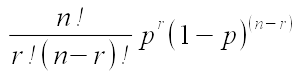

 ), and for
the "Bounds" set the minimum to 0 and the maximum to 25 for the y-axis - note that you MUST ENTER THESE VALUES,
even if they are already at 0 and 25, because entering them prevents the axis from auto-scaling as the data
changes. If you did it correctly there will be a box that says "Reset" next to the minimum and maximum bounds.
), and for
the "Bounds" set the minimum to 0 and the maximum to 25 for the y-axis - note that you MUST ENTER THESE VALUES,
even if they are already at 0 and 25, because entering them prevents the axis from auto-scaling as the data
changes. If you did it correctly there will be a box that says "Reset" next to the minimum and maximum bounds.