Estimating population size with more than two captures

Now that you have had some experience with likelihood-based population size estimation, we can move on to the more informative case in which we have three capture periods. We are still going to assume demographic and geographic closure, so this approach is still best for studies that cover brief periods of time. However, by adding just one more capture period we gain enough degrees of freedom to start asking some important questions about how our sampling is working. Specifically, we can assess whether encounter probability is the same in each trapping period, or whether the chances of re-capturing the lizards are different than the initial probability of capture.

Let's start by getting an idea of how this will work - we have three different models that explain our encounter histories below, each one showing the observed data (in blue) plus the estimated frequency of the 000 history (light blue), along with the expected frequencies (in orange). Like our first time working with these capture models, expected frequencies are total number of individuals (that is, the sum of the observed captures plus the estimate for the number never captured, f(000)) multiplied by the probability of the capture history.

At first, all of the parameters are set to the same values, so the graphs are identical. Model M₀ has a single probability of capture, so the probability of each history is obtained by multiplying either p or (1-p) together, given the 0's and 1's in the history - that is, history 001 is (1-p)(1-p)p, and history 110 is pp(1-p). Model M_t hypothesizes that the probability of encounter was different at each capture, so we have a p₁, p₂, and p₃ to represent these probabilities, and under model Mt history 001 has probability (1-p₁)(1-p₂)p₃, while history 110 has probability p₁p₂(1-p₃). Model M_b hypothesizes that the animals change their probability of capture after they are captured the first time (either by becoming easier to capture or harder to capture, depending on how nice we've been to them), such that we have a probability p for the first capture, and c for captures after the first. With Mb the probability of 001 is (1-p)(1-p)p, and for 110 is pc(1-c).

The initial choices for capture probabilities and f(000) are all the same, and all pretty bad - the observed and expected bars are pretty far apart. As before, the closer the observed and expected values get the higher the log likelihood. As you change the values for the p's and f(000) the color of the graph title and log likelihood changes, from black to red, as you get the bars closer together - as you get close to the maximum likelihood the color turns bright red (you can also watch the values reported for the log likelihood, which you want to make as big as possible). Bear in mind that the ML estimates of any single parameter depends on the values of the other parameters in the model, so if you just change one of the parameters until you get the likelihood as big as possible and then move on to the next, after you have gotten the likelihood as high as possible by changing the second parameter you may be able to do better still by going back to the first one and changing it again. As a hint, all the capture probabilities are around 0.25, and the frequency of animals never caught is 108 or more for all of the models.

When you get them all as close as you can, you'll see a couple of important things.

First, you'll see that the estimated frequency of the 000 capture history is different for all three models, which means that the estimated population size (N̂) is also different. Since they all produce different estimated population sizes we need to find out which model fits the data best so that we know which estimate of N̂ to use.

Second, the model with the highest likelihood is the M_t model, but that's alone is not justification to treat it as the best model, because it is also the one with the most parameters. Having the ability to adjust the probability of capture for each time points allows the model to fit the data more closely, but that would be true even if the probability of capture was actually always the same every year - the number of animals captured would be at least a little different every month just due to random chance, but having a p that is different each month would allow the predicted values to come closer to the observed captures, which would increase the likelihood of that model. The more complex model could just be describing random variation rather than real changes in capture probability - this is referred to as over-fitting. We need to balance the fit of the models (as indicated by the log likelihood) against each model's complexity (as indicated by the number of parameters they each contain) in order to find the model that is best supported by the data while avoiding over-fitting.

We will analyze these data in Excel so that we can compare the models against each other once we have found the maximum likelihood estimates for the parameters, and identify which model to use to estimate population size.

Model M₀ - constant encounter probability

Let's get our first set of estimates, with constant capture probability, and then we'll consider what questions we might want to ask about our data.

1. Open your Excel file from last time, and switch to sheet Mo. You'll see that, in the interest of time, I've done some work for you.

• I used the original capture histories in the Captures sheet to tabulate frequencies of all seven of the possible observable capture histories, and added a label for the one that can't be observed, 000. I used the same procedure you used for your ML estimates for two capture periods, just with all three months of data included.

• With a constant encounter probability assumed, we just need one encounter probability, p, which has its MLE in cell E2, based on the sin link function (the beta for the link function is in cell F2).

• The MLE for the unobserved frequency of 000 is calculated in cell E7 with a log link, using a beta in cell F7.

• The estimate of population size, N-hat, is in cell E9.

• All of the LnLikelihood calculations are in cells A11 through D12. These calculations are exactly the same as you did for two capture periods, only the numbers are different. The probability part and LnLikelihood are both showing errors for now because you haven't calculated the multinomial probabilities - that's going to change shortly.

• Space for the multinomial probabilities are in column H, and expected frequencies will calculate automatically in column I.

All you will need to do is calculate the multinomial probabilities of each history, and run Solver to get your estimates.

2. Calculate the multinomial probabilities. The only difference from what we did last week is that the probabilities are now due to three capture periods instead of two. The first History in the list is 001, which means it was not observed the first time (at a probability of (1-p)), was not observed the second time (at a probability of (1-p)), and was observed the third time (at a probability of p). You can enter this probability into H2 as =(1-e2)*(1-e2)*e2.

You should now be able to do the probabilities for the rest, based on the histories. Don't forget the 000 history. If all goes well your probabilities should look like this (to three decimal places):

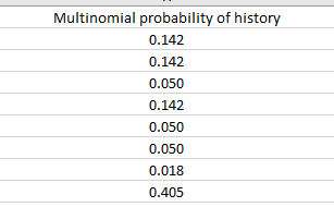
When you're done, check that the eight probabilities you calculated sum to 1 - if you select the cells H2:H9 Excel will show the sum in the status bar at the bottom of the spreadsheet -  the sum of the multinomial probabilities should be 1. If not, you did something wrong - check your calculations. If you can't find the error send up a distress signal and I'll help you.

All of the LnLikelihood statistics should have updated when you calculated your miltinomial probabilities, so you should be all set to go.

3. Get your estimates for p and f(000). Start up Solver, and set D12 to maximize by changing F2 and F7 (remember that you want to change the betas, not the estimates directly).

Once you have your estimates for p and f(000) cell D9 will have the estimated population size.

The Expected column (I) is the N-hat estimate multiplied by the multinomial probability of each history. A model that matches the data well will have observed frequencies (in cells B2 through B8) that match the expected frequencies closely, so look at these to get an idea of how things are working (the interactive graphs above are graphing these, so once you get your estimates for p and f(000) you can enter those values above to get a graph of the result).

A single likelihood doesn't tell us much - the value should be 452.09, but we have no way of knowing if that is good or bad. To interpret likelihoods we need to compare them to other likelihoods, so we now need to find the ML estimates for the other two models and then compare the likelihoods of all three together.

So, now we're cooking with gas. Time to make things interesting.

Model M_t - encounter probability that changes over time

Switch to sheet Mt. You'll see the layout is almost the same as Mo, except that we have three encounter probability parameters, p1, p2, and p3, which are the encounter probabilities for the first, second, and third capture periods, respectively. To get estimates for these, as well as the frequency of 000 in cell E7, you just need to calculate the multinomial probabilities and run the Solver.

1. Calculate the multinomial probabilities. The first history is 001, and since we now have a different probability for each capture period, its probability will be (1-p1)*(1-p2)*p3. Since p1 is in cell E2, p2 is in cell E3, and p3 is in cell E4, the formula for this will be =(1-e2)*(1-e3)*e4.

Try the rest yourself. With the betas all set to -0.5 for the probabilities the probabilities of the histories will be the same for all the models before you get your estimates, so check that the numbers match thee ones for M₀, above, and sum to 1.

2. Run Solver to get your estimates. Once you have the probabilities right, the rest of the spreadsheet is all ready for fitting (there is no change to the likelihood function itself, so the rest of the cells correctly updated to reflect the new probabilities). You can now run Solver, but make sure you set it to vary cells F2:F4 as well as F7 so that all three capture probabilities will be estimated.

Model M_b - response to capture

Model Mb is the "behavior" model, because it models a response to trapping (being "trap happy" or "trap shy"). But, as we discussed in lecture, differences can be due to more than a behavioral change by the animal - it can be due to a difference in detection method for the first and subsequent captures, which could happen if the first detection is done by trapping and marking the animals, whereas later "captures" are actually resightings with binoculars. Any time there might be a difference in encounter probability between the first and subsequent captures we can use model Mb.

In any event, model Mb assumes that the probability of encounter isn't dependent on time, but that after the first capture the probability of encounter changes.

1. Calculate the multinomial probabilities. Switch to sheet Mo, and you'll see again that the difference is in the encounter probabilities. Now, we have a single p, indicating the probability of first encounter, and c, indicating the probability of subsequent encounters. Use these to calculate the multinomial probabilities of the capture histories, and you'll be ready to run Solver to get your estimates. For example:

• The first history of 001 was first captured in the last capture period, and thus no recaptures, so it will have a probability of (1-p)*(1-p)*p. The formula is =(1-e2)*(1-e2)*e2.
• The next history is 010, so it had a first capture in the second capture period, and was not captures in the last one. The probability for this history is thus (1-p)*p*(1-c). Why did we use (1-c) for the last non-capture? Because, once the animal has been captured then the probability of being caught again is c, and if the animal is not recaptured the probability is (1-c). So, the Excel spreadsheet formula is =(1-e2)*e2*(1-e3).

Go ahead and try the rest yourself - check that the probabilities sum to 1 before you run Solver. They should match the probabilities you got initially for the other two models (see screen shot for M₀, above), and should sum to 1.

2. Run Solver, and obtain the estimates.  Run Solver, but this time only change the betas in F2, F3, and F7.

Testing hypotheses about our study: Comparing models M₀, M_t and M_b.

Now we need to find out which of the three models we have fit that is best supported by the data. We will calculate AICc values for each model, and use them to pick the one that best balances model fit against model complexity.

We have compared models to one another once before, when we compared the polynomial regressions for species of raptors counted at Hawk Mountain, and for those comparisons we calculated F tests, and used the p-value to decide if adding a higher polynomial term increased fit. Those sorts of model comparison are only appropriate for "nested" models, in which one model has a subset of the terms found in the other - when we were comparing a linear model to a quadratic model the quadratic had a linear term as well as a quadratic, so the linear model was a nested subset of the quadratic. That isn't true here, we have different parameters in each model, so we need to use a method like AICc that can handle non-nested models.

1. Record -2LnLikelihood and number of parameters for each model in sheet AIC. If you switch to sheet AIC, you'll see a blank table with a row for each model we will compare: Mo, Mt, and Mb. This is where we will do the calculations necessary to determine which model is best supported by the data. Most of the entries in the table will be calculated, but we to record the LnLikelihood (multiplied by -2) and the number of parameters estimated for each model.

• In cell B2, type =-2*, and then before hitting ENTER, switch to sheet Mo and click on cell D12 - the formula should say =-2*$Mo.D12 , which is a reference to cell D12 in sheet Mo. Now hit ENTER - this is the log-likelihood part of AIC.

• In sheet AIC, enter the number of parameters estimated for model Mo - there is one encounter probability, and the frequency of 000, so there are two parameters. Enter a 2 under the K in column C (cell C2).

• Repeat this process for Mt and Mb. Calculate -2*logLikelihood for each, and for K:
• There were four parameters estimated for Mt (p1, p2, p3, and f(000)) - use 4 for K
• There were three parameters for Mb (p, c, and f(000)) - use 3 for K

2. Calculate AIC. AIC is just -2LnLikelihood + 2K, so in cell D2 type =b2+2*c2. Copy and paste this to cells D3 and D4.

3. Calculate AICc. With a small number of captures per parameter it's best to use AICc, which takes the AIC you just calculated and adds an additional penalty for the number of parameters in the model. The formula is AIC + 2K(K+1)/(n-K-1).

In cell E2 type the formula =d2 + 2*c2*(c2+1)/(185-c2-1). The 185 used for n is the total number of animals captured.

Copy cell E2 and paste it to cells E3 and E4.

4. Calculate ΔAICc. In cell F2 type =e2 - min(e$2:e$4). Copy and paste this to the other two rows.

The raw AICc values are hard to interpret, but these deltas can be interpreted more easily. The model with a 0 is the best supported, and deltas up to 4 are considered to have good to moderate support in the data. Deltas over 10 have essentially no support.

We can use the Akaike weights to give us a more probabilistic interpretation of these deltas, which we'll calculate next.

5. Calculate the weights. In cell G2 type =exp(-f2/2)/sum(exp(-f$2:f$4/2)), and hold down CTRL+SHIFT when you hit Enter to make this an array formula. Copy and paste this to cell G3 and G4 (this is a case where you should NOT use the fill handle - it does unexpected things with array formulas).

Your completed AIC table should look like this:

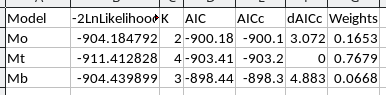
6. Interpret the results. Take a look at the dAICc values and see which model is best supported. We would like to see a clearly best model, but you may not - if there are deltas less than 4 then more than one model is well supported by the data, and we should interpret any with good support.

Based on what you find, interpret the models with good support. What are the population size estimates? If there is evidence of encounter probabilities that are not always the same, how did they differ (is it Mt, or Mb, or possibly either)?

That's it! Save a copy of your Excel sheet, you'll need it for your report.