Today we will compare the density estimates obtained using fixed width
transects and using distance sampling.
Fixed width sampling is the simpler method - an observer walks a
transect, and counts all of the individuals observed within a fixed
distance of the line. The area sampled is simply the length of the line
multiplied by twice the distance:
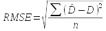
Consider this
example - the green circles are coast horned lizards for which we want a
density estimate. The black line is the transect line we would walk along,
and it is 100 m long. We would record every lizard within 5 m of the line,
so the area surveyed is:
A = 100 x 5 x 2 = 1000 m2
Within this fixed width transect there are 14 lizards, so the density of
lizards would be estimated as:
D̂ = n / A = 14/1000 = 0.014 lizards per square meter
To express this as lizards per hectare, we could multiply by the number
of square meters per hectare (10000), which gives us the estimate as 140
lizards per hectare.
The problem with fixed-width samples, however, is that they assume that
every individual that is within the transect is detected. This is probably
reasonable if the transect width is narrow, but as the width of the
transect increases it becomes increasingly unlikely to be true. If some of
the individuals in the transect are missed the density estimate will be
biased low, so to be effective fixed-width transects have to be narrow.
But, narrow transects sample a smaller area for a given transect length.
A small area sampled means few lizards detected, which would lead to
variable, imprecise estimates of density.
Distance sampling solves the detectability problem by modeling changes in
detectability with increasing distance. In distance sampling, every
individual detected is counted, and its perpendicular distance from the
line is also measured, but it is assumed that not every individual present
was actually seen.
The distribution of detection distances is used to measure the change in
detectability with distance. The line fitted to the distribution of
distances in the graph to the left illustrates the approach - if the
actual density is constant throughout the region then the decline in
numbers of detections with distance is purely due to a change in
detectability, so once we know how detectability changes we can adjust for
the animals not seen.
The equation for the population density estimate is ; n is the number of individuals counted,
and L is the length of the transect. The detection function is f(x), and
f(0) refers to the value of the function when 0 is plugged in (in other
words, f(0) is f(x) evaluated at 0). The detection function evaluated at
zero is the inverse of the effective width, which refers
to the equivalent width of a fixed-width transect sampled with perfect
detectability. If f(0) is the inverse of the effective width, then is the estimate of effective width.
Using effective width instead of f(0) makes the estimator , which looks just like the
formula for density in a fixed width transect, except that effective width
is used in place of the fixed width of the transect. Distance sampling
estimates the curve that describes the reduction in detectability with
distance, uses it to estimate effective width, and then calculates the
density from the number of individuals observed, the length of the
transect, and the effective width.
Distance sampling is great stuff - it's clever and sophisticated, and
improves on fixed width estimates. However, like any estimation method, it
makes some assumptions:
Detection probability is assumed to be 1 at a distance of 0 - in other
words, if a lizard is right on the line it will be detected. This isn't
always true; species that dive under water, or hide in burrows, or are
very cryptic and difficult to see could go undetected as you move right
over them. If you know this is the case and can estimate the probability
of detecting individuals right on the line you can correct for this, but
otherwise the method under-estimates the actual density (so would fixed
width samples, but still).
Density is homogeneous throughout the area surveyed - no moving
between habitats, no gradients in population density from one end of the
transect to the other, and the transect is in the same habitat for its
entire length.
The detection function fits the data well, meaning that it describes
the decline in detectability accurately - but, it doesn't have to fit
too well to improve on fixed width estimates. Correcting for the dropoff
in detectability with distance is good, even if it is done imperfectly.
The app I wrote for you uses the positive side of the normal
distribution.
Today's activity
I put together a simulation for you to use, which can open in a separate
window by clicking here.
Once the link opens, you will see a blank table of density estimates at
the top, and a map of an area of California desert somewhere not too far
from here.
The transect length is set initially to 100 (m) and the distance visible
is set to 20 (m). When you click the "Select transect" button for the
first time a transect 100 m long is placed on the map, and the horned
lizards detected are shown as colored dots.
Red dots are horned lizards detected with distance sampling
The number of lizards detected by distance sampling is in row n
under the Dist. column.
A curve is fitted to the distances for the detected lizards by the
app, and the curve is used to calculate f(0). From f(0) the effective
width of the transect is calculated, and is reported in the sub-title
of the graph.
Density is calculated as number detected divided by effective width
x transect length, which is then multiplied by 10,000 to convert to
number per hectare. This estimated density is in the Density row.
The green dots are lizards that were detected in a fixed-width
transect 5 m on either side of the line (10 m wide total).
All of the lizards in this transect are detected, and are in the n
row of the FW column.
Density is based on the count of lizards detected divided by 10 x
transect length, which is then multiplied by 10,000 to convert to
number of lizards per hectare. This is reported in in the Density row.
The histogram shows the distribution of distances from the line for
the lizards detected, with the curve overlaid. The effective width,
which is 1/f(0), is displayed in the graph sub-title.
If you click on the "Select transect" button a second time, you'll see
that a new transect is selected, with a new distance sample and a new
fixed width sample. The density estimates update to reflect this new
sample.
There are two properties of the sampling that you can change:
The maximum distance that individuals are detectable - changing the
distance detectable only affects the distance sampling estimates,
because the fixed width sampling is always set to 10 m in this
simulation.
The length of the transect - changing the length of the transect
affects both distance sampling and fixed width sampling.
The activity for today is to try out a range of detection distances, and
a range of transect lengths, and see how distance sampling estimates and
fixed width transect estimates compare. Download this
worksheet to your S: drive, and use it to record your results.
You'll see that the Data worksheet is already laid out for you with
lengths of transects and distances, you just need to fill in with survey
results.
1. Varying detection distance. Keeping the length of
transect at 100, with the Distance detectable to 20 m, click "Select
transect" and record the five statistics for this combination of distance
and transect length in your worksheet. The button below the table of
density estimates, labeled "Copy estimates", copies all of the things you
need to record for each run in a format that can be pasted directly into
the spreadsheet, so all you will need to do is to set the transect lengths
and detection distances to values given below, select the transect, and
then copy and paste the values into Excel.
Repeat four more times at 20 m, and then repeat the process for detection
distances of:
50
100
As you are working through this part of the activity watch the histogram
on the left side of the simulation - you should see that more lizards are
detected as your visibility increases, and this gives you a better match
between the bars of the histogram and the detection function. Given how
important that detection function is to a distance sampling estimate of
density, you might anticipate better estimates as the visibility
increases.
Before you move on, think about detectability - we are able to set
detection distance to any value we want in a simulation like this one, but
how much control would you have over it in nature? You can influence
detectability through your sampling methods - you can use binoculars, you
can survey when the animals are most active (dawn for songbirds, nighttime
for frogs, etc.), you can avoid days with poor visibility (high wind,
rain, fog, etc.). However, detectability is also strongly influenced by
factors that are beyond your control, like environmental conditions
(whether the area is heavily vegetated, whether there are leaves on the
trees) and by how cryptic the organisms you're surveying are.
2. Varying transect length. Set the detection distance
back to 20 m, and set the transect length to 200 m. Generate 5 transects
for 20 m detection distance, then 5 for 50 m detection distance, and 5 for
100 m detection distance. Remember to copy the estimates and paste them
into your Excel sheet each time (if you start seeing duplicated rows you
forgot to copy the estimates before pasting - don't ask how I know that -
so generate a new transect and copy/paste over one of the duplicates if
this happens to you).
Then set the transect length to 400 m, and then use the 20, 50, and 100 m
detection distances for that transect length (five each).
Again, watch the histogram - longer transects will give you more points
at a given detection distance. The n.fw values go up as well. You might
thus expect longer transects will give you better estimates.
Keep in mind that this is actually the parameter you have the most
control over when you are monitoring. The length of the transect is an
investigator's choice, within limits. For example, longer transects are
more likely to cross over into a different habitat that has a different
density of organisms, which would run afoul of the constant density
assumption. There may also be boundaries on the study area or barriers to
movement that can't be gotten around. But, within these broad constraints,
any transect length can be used.
3. Squared differences from true density. Once you have
your results in your Excel spreadsheet (which you should SAVE NOW), you
need to do two more calculations before you can analyze the data. We know
what the actual density of dots on the map is, and we need to assess how
close our estimates were to the correct number. We will calculate a
statistic called the "root mean square error", or RMSE, to measure this.
The calculation is like a standard deviation, but we use the known density
instead of the mean of the data:
The hat-D's are the estimates, and D is the known density. The formula
calculates the average of the squared differences between the estimates
and the true value, and then takes the square root of the average. There
are 9600 animals (mostly hidden) on a map that is 1200 m by 1600 m, or
9600/(1200x1600) = 0.005 lizards per square meter. Multiplying by 10,000 m2/ha
gives us 50 lizards per hectare - this is the true value
of density, D. We will use PivotTables to calculate the averages, so for
now we just need the squared differences for each of our estimates.
In cell H1 type "Density.sqdiff", and in cell i1 type "FW.sqdiff". In H2
enter the formula:
=(d2-50)^2
and in I2 enter:
=(g2-50)^2
Copy and paste cells H2 and i2 down to the rest of the rows. Now you're
ready for some pivot tables.
4. Summarizing distance sampling density estimates with a
PivotTable. Select cell A1, and insert a PivotTable. Let Excel
put the table in a new worksheet.
We'll do the distance sampling data first:
Put "Length of transect" into the rows
Put "Distance" into the columns
Drag Density.dist into the Σ values, and change the value field to
Average. These are the average density estimates for your five
replicates at each combination of distance and transect length.
Once you have your new worksheet with your PivotTable, change the name of
the new worksheet to "Pivot" (double-click on its tab and change the name
to Pivot).
5. Summarizing fixed width sampling estimates with a PivotTable.
Switch back to sheet Data. Select cell A1 again, and insert another
PivotTable, but this time use the Existing Worksheet option and put it in
the Pivot worksheet, in cell A15.
Drag the Length of transect into the Rows, but this time don't bother
with the Distance column - detection distance wasn't part of fixed width
transect estimates, so we don't need to account for it here.
Drag Density.fw into the Σ values area, and change the value field to
an Average. These are the average densities for fixed width sampling.
6. Collect results. We will be making several different
PivotTables, so we need to record results - add a new worksheet, and
change its name to "Results".
Back in sheet Pivot, select the first PivotTable in cells A3 through E8,
copy, and paste special as values in the Results sheet in cell A5. In cell
A1 enter the label "Distance sampling", and in cell A3 type "Average
density".
Switch to Pivot, copy your fixed width density estimates from A15 to B19,
switch to Results and paste-special as values to cell H6. In cell H1 type
"Fixed width transect".
You can change the label in cells A6 and H6 to "Transect length" (do this
for each of the pivot tables you put into Results).
7. Number of lizards detected. Back to sheet Pivot.
Keep the same layout for each pivot table, but take out the densities, and
put in the number of points detected - this will be n.dist for the
distance sampling pivot table, and n.fw for the fixed width transect pivot
table. Set the value fields to calculate averages.
Copy and paste-special the values for the distance sampling pivot table,
into the Results sheet in cell A14. Type "Number of points" in cell A12.
Copy and paste-special the fixed width pivot table into cell H15.
8. Effective width of distance samples. Back in sheet
Pivot, calculate the average effective width for distance sampling - take
out the n.dist field from Σ values, and put in Eff.width.dist. Change it
to an average.
Copy and paste this table to Results, cell A23. Enter "Effective width"
in cell A21. We didn't need to estimate an effective width for fixed width
sampling, because the width was always 10 m.
9. RMSE of estimates. Back in sheet Pivot, take out
Eff.width.dist from Σ values, and put in Density.sqdiff, and change it to
an average. Do the same for fixed width - take out n.fw, and put in
FW.sqdiff and change it to an average. Copy the distance sampling table
from Pivot, and paste-special as values in Results cell A32. Copy the
fixed width table and paste-special in cell H33 of Results.
Enter the label "Mean squared differences" in cell A30.
We're not quite done with this calculation though - we need square roots
of these values.
So, in cell A39 enter "Root mean square error". We will want to use the
same layout as the tables we have been copying and pasting, so as a
convenient way to get the layout all at once copy the mean squared
difference table (cells A32 to E37), and paste it into A41.
Then, in the first cell of data (B43) enter the formula =sqrt(b34) - this
will take the square root of the mean squared error from B34. Copy and
paste this cell to the rest of the cells in the table to complete the RMSE
calculation for distance sampling.
Do the same for fixed width - copy the table from H33 to I37, paste it to
H42, and then replace the table entries with formulas that calculate the
square roots.
10. Graph the results. To make the comparison between
the methods easier, we need to graph each of the results. The names on the
graph will come from column names, so change the fixed width column labels
to FW for all of the results in column I (cells I6, I15, and I42).
Then to make a graph of the average densities, do the following:
Change the length of transects to text, so that they will be used as
labels - enter an apostrophe before each number, and when you hit ENTER
it will left-justify and gain a little green triangle in the upper left
corner indicating it is now text.
Select the cells from A6 to D9, hold down the CTRL key and select
cells i6 to i9.
Insert a line graph with both lines and dots (line graphs have a
categorical x-axis, which is what we will be using here).
Select one of the lines, right-click and select "Select data"
Switch the rows and columns so that transect lengths are on the
x-axis, and detection distances and FW are the four data series
Change the chart title to "Estimates"
Add axis labels, and change the x-axis to "Transect length", and the
y-axis to "Density"
You'll see that all of the methods give fairly consistent estimates of
density on average. This shows that both of the methods are unbiased.
Repeat these steps to get graphs of:
Number of points
The y-axis will be "Number of points", and the title should be
"Number of points".
Look at how extending the transect length increases the number of
points detected for both methods, and how increasing the detection
distance increases the number of points detected for distance
sampling. The number of points detected is a major determinant of the
precision of estimates, so distance sampling has a big advantage in
this regard.
Effective width
Effective width only pertains to distance sampling, so you only need
to select the distance sampling columns.
Since we don't have a FW column for this graph Excel gets confused
and doesn't realize the first row are labels, so we need to convert
them to text. Add an apostrophe before the visibility numbers, '20,
'50 and '100 - otherwise, use the same steps as for the other graphs.
The y-axis title and chart title are "Effective width". You should
see that the transect length doesn't have much effect on effective
width (the lines should be pretty flat), but the longer the detection
distances the wider the effective width. Fixed width transects are
always the same width (10 m in this example).
RMSE
The x-axis label is "Transect length", and the y-axis and chart
title should be "RMSE"
RMSE is comparing the estimates to the true density - smaller values
are better precision. If you see from your chart of average densities
that the values are close to 50 on average, but that the method has a
high RMSE, that should tell you that the method is accurate but not
precise. You should see that distance sampling is not better than
fixed-width sampling (and may even be worse) with 20 m detection
distances, but with longer detection distances it gives more
consistent estimates, with lower RMSE, than fixed-width samples. If
you look at the number of points graph, you get similar numbers of
points with distance sampling and fixed-width sampling with a small
detection distance, so better precision is not to be expected. With
bigger detection distances the number of points detected increases,
and distance sampling begins to out-perform fixed-width sampling.
You should see that distance sampling does better than fixed width
sampling usually, particularly when the detection distance is 50 or 100.
You should also see that increasing the transect length is generally a
good thing for the accuracy of your samples - the RMSE tends to go down
with increasing transect length for both methods, because longer transects
mean more detections (your graph of detections should show an increase as
the transect length increases, or as the detectability increases).
It's difficult to tell with just one set of estimates, but both distance
sampling and fixed width sampling is unbiased - the estimates are correct
on average. Your estimated densities should be around 50 for both methods
at all transect lengths and detection distances. What changes is the
variability in the estimates, and there distance sampling is usually
better.
That's it! Save your work, you'll need it for the final project write-up.
 Consider this
example - the green circles are coast horned lizards for which we want a
density estimate. The black line is the transect line we would walk along,
and it is 100 m long. We would record every lizard within 5 m of the line,
so the area surveyed is:
Consider this
example - the green circles are coast horned lizards for which we want a
density estimate. The black line is the transect line we would walk along,
and it is 100 m long. We would record every lizard within 5 m of the line,
so the area surveyed is: 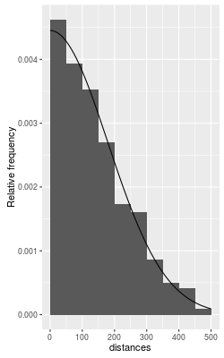 Distance sampling solves the detectability problem by modeling changes in
detectability with increasing distance. In distance sampling, every
individual detected is counted, and its perpendicular distance from the
line is also measured, but it is assumed that not every individual present
was actually seen.
Distance sampling solves the detectability problem by modeling changes in
detectability with increasing distance. In distance sampling, every
individual detected is counted, and its perpendicular distance from the
line is also measured, but it is assumed that not every individual present
was actually seen. ; n is the number of individuals counted,
and L is the length of the transect. The detection function is f(x), and
f(0) refers to the value of the function when 0 is plugged in (in other
words, f(0) is f(x) evaluated at 0). The detection function evaluated at
zero is the inverse of the effective width, which refers
to the equivalent width of a fixed-width transect sampled with perfect
detectability. If f(0) is the inverse of the effective width, then
; n is the number of individuals counted,
and L is the length of the transect. The detection function is f(x), and
f(0) refers to the value of the function when 0 is plugged in (in other
words, f(0) is f(x) evaluated at 0). The detection function evaluated at
zero is the inverse of the effective width, which refers
to the equivalent width of a fixed-width transect sampled with perfect
detectability. If f(0) is the inverse of the effective width, then  is the estimate of effective width.
  , which looks just like the
formula for density in a fixed width transect, except that effective width
is used in place of the fixed width of the transect. Distance sampling
estimates the curve that describes the reduction in detectability with
distance, uses it to estimate effective width, and then calculates the
density from the number of individuals observed, the length of the
transect, and the effective width.
, which looks just like the
formula for density in a fixed width transect, except that effective width
is used in place of the fixed width of the transect. Distance sampling
estimates the curve that describes the reduction in detectability with
distance, uses it to estimate effective width, and then calculates the
density from the number of individuals observed, the length of the
transect, and the effective width.