Lab 16 - estimating reproductive parameters in birds

Reproduction is estimated with a variety of methods for different species. Species that develop embryos internally (gestation) are more difficult to assess at early stages, and estimates of reproduction are either based on dissection of a sample of females (e.g. counts of placental scars, corpora lutea), or by using portable x-ray or ultrasound equipment on live animals. After birth it is possible to survey populations to count offspring, and ratios of offspring to total individuals, or total females, or total females of reproductive age can be used to assess the reproductive output for that year.

Compared with all of that, measuring reproduction in birds is a breeze. Since they lay eggs, measuring reproduction is just a matter of finding nests and counting how many eggs are laid, how many hatch, and how many leave the nest (i.e. fledge, which makes the newly independent youngsters fledglings).

The variable that is most important to population dynamics is the average number fledged - fledging is the point at which the chicks are recruited into the population. However, fledging is the end of a series of positive outcomes, each of which are subject to different environmental conditions. For a chick to eventually leave the nest, first a pair of adults has to form, and establish a breeding territory. Then they need to build a nest and lay eggs in it. Then the eggs need to hatch successfully. The parents need to be able to find enough food in the vicinity of the nest to feed the growing nestlings until they are ready to fledge and start foraging for themselves. Recording various stages of the breeding cycle helps biologists identify what problems, if any, the species is experiencing in its reproduction, and to identify possible causes for the problems. For example, up to the point that eggs are laid it will be environmental factors that act on the parents that matter - the parents have to be healthy and well fed enough to build a nest and lay eggs. Once the eggs are laid then other factors come into play, such as nest predation and food levels - even in species that are herbivorous as adults feed their chicks animal foods (often arthropods), and the availability of the adult's food may not be the same as availability of the foods they will feed their chicks. If pairs establish territories and lay eggs in large numbers only to have the chicks starve to death, this is a very different situation than if the parents are too poorly fed to initiate breeding in the first place. Measuring reproduction in multiple ways is thus not being redundant, it is an important way to better understand the factors that are limiting a population's reproductive output.

Ravens in the West Mojave Desert

We will be working today with a data set my colleagues and I collected on breeding biology of the Common Raven (Corvus corax) in the west Mojave Desert. The study was funded by Edwards Air Force Base (EAFB), because ravens were using their landfill as a food source and their buildings as nesting areas, and the US Fish and Wildlife Service was concerned that the unnaturally high population of ravens on and near the base may be affecting desert tortoise populations.

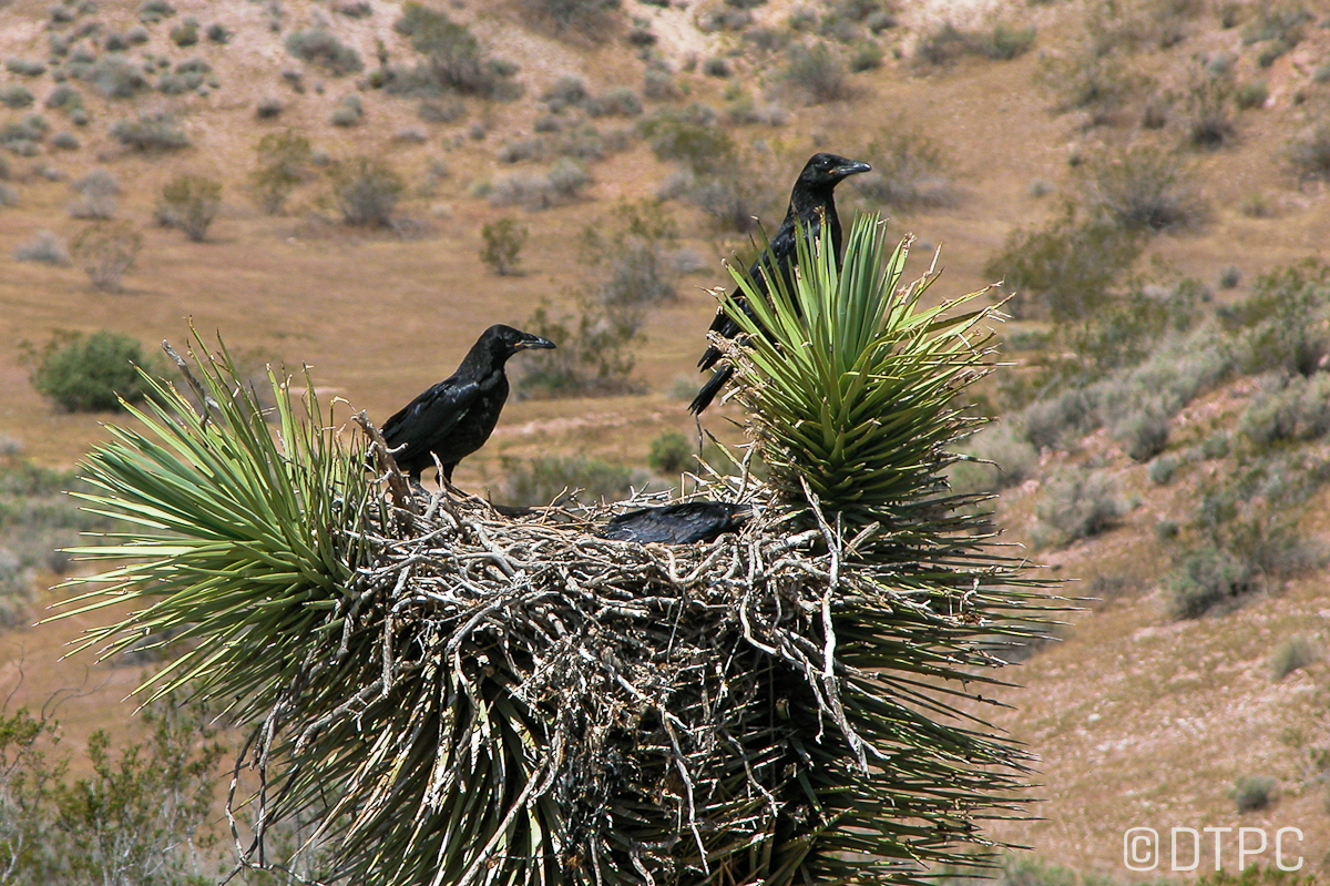
Ravens place their nests on a wide range of structures (or "substrates"), including Joshua trees where they are available.

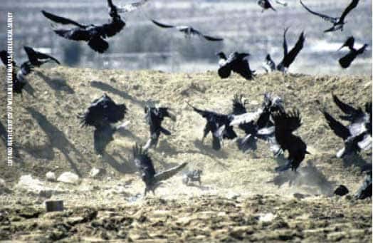
Ravens have a reputation for being scavengers, like these birds at the EAFB landfill, and they are. In addition to garbage they also use road-killed carrion, which allows them to eat animals that would be too large for them to kill themselves.

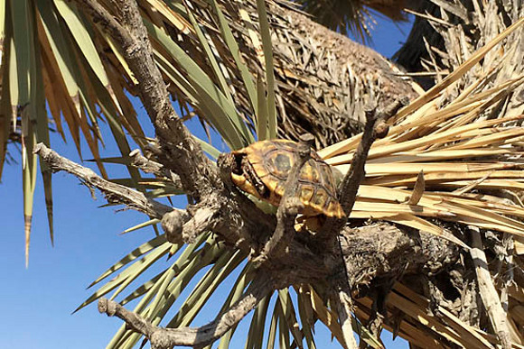But they are also capable of hunting small animals, and are able to peck through the shell of juvenile desert tortoises - desert tortoises don't climb Joshua trees, so finding a shell with a hole in its back up in a Joshua tree is pretty compelling evidence of raven predation.

Ravens and tortoises are both native species, and have both been in the Mojave desert for a very long time. Raven predation has probably not been common enough in the past to be a problem - ravens are generalist species found all over North America, and are not especially well adapted to the desert, and were probably always fairly uncommon. However, as people developed the desert they started providing ravens with the resources they need to reach large population sizes, to the point that they pose a threat to desert tortoise populations.

The project I worked on studied the three-way relationship between people, ravens, and desert tortoises. The link between people and raven reproduction was part of that set of interactions, and the nesting data we will work with today comes from the two years that I worked on that study.

If you download this file and open it, you'll see that it is a spreadsheet with the data presented in two different formats. The tab repro_data_raw sheet shows the data with a single row for each nest in each year for each measure of reproduction. This is already actually summarized data, because the raw data would have included weekly checks of the known territories and active nests, so there would have been multiple weeks of data for each nest that were used to get these final values.

The worksheet we will use for this exercise is repro_data. You can see it has a row for each raven nest made during two breeding seasons, 1999 and 2000, arranged with the following columns:

Year = the year of observation.
nest.id = the unique identifier for a single nest. Nests could be used by ravens for multiple years, and tended to persist for multiple years even if they weren't being used.

Occupancy = whether a known territory was occupied. Possible values are 0 (not occupied) or 1 (occupied)

Initiation = whether breeding was initiated. The possible values are 0 (not initiated) or 1 (initiated).

Clutch = number of eggs observed in the nest

Chick = number of chicks observed in the nest

Fledge = number of chicks fledged.

The repro_data worksheet was obtained from a PivotTable of the raw data, but the data are the same.

To use the data in repro_data to assess the reproduction of ravens in these two years, we will be calculating the following:

Occupancy rate = the proportion of known territories occupied each year.
Initiation rate = the proportion of occupied territories in which breeding was initiated
Average clutch size = for the nests in which eggs were laid, the average number of eggs observed
Hatching success = the average proportion of eggs that hatched a chick
Proportion of nests that fledge = the proportion of nests with initiated breeding that fledged at least one chick
Average number of chicks fledged expressed as:

Average number fledged per occupied territory = occupied territories are our measure of the number of potentially breeding females.
Average number fledged per female that initiated breeding = this is an estimate of reproductive output for females that initiated breeding, and/or were observed with at least one egg or chick during the breeding season.

You'll see that some of these measures are proportions and some are averages - the confidence interval calculations are a little different, as you will see. The actual calculations involved are simple arithmetic. The complicated part of doing the calculations is in summarizing the data properly, so that the rates can be calculated accurately.

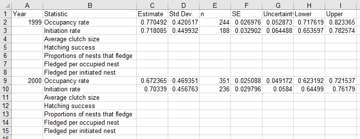
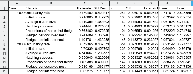
1. Switch to the Estimates sheet and you will see a table laid out like this:

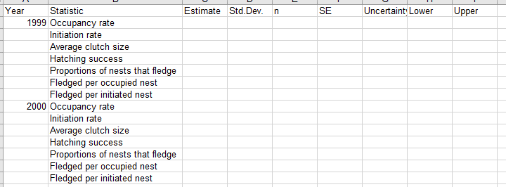
You will be calculating the estimates for each of these reproductive measures, and then calculating their 95% confidence intervals.

2. To obtain these measures, you need to make a PivotTable of the data.

Select a cell in the data set in sheet repro_data, and allow the PivotTable to start a new worksheet.
Use Year as the COLUMNS
Use Nest.ID for the rows.
Use Occupancy for the VALUES - change it from a Count to Average.

Your table will look like this:

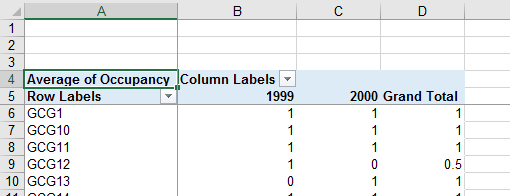
Notice that since the entries in Occupancy are either 0's or 1's, summing these gives a count of how many occupied territories there are, and dividing by the sample size thus gives you the number occupied divided by the total number of nests.

Okay, before we move on, let's look at how excel does calculations when there are blank cells...

The data has an important feature we have to be aware of. If you look at any of the columns in your pivot table, you'll see that sometimes there are blanks, and sometimes there are 0's. These are not the same thing.

Blanks are missing values. If you look at the data for 1999, you will see there are cases in which there are blanks for the Occupancy column, but values recorded for Initiation. When this happened it was because the nest was originally found in 1999, but was found late enough in the season that the birds were already engaged in breeding activity. In principle it was possible to fill in the blanks for those nests, because a nest had to have been occupied before breeding could be initiated, but we decided not to do this because territories with breeding pairs are much easier to locate than ones in which breeding is never initiated. If we filled in the blanks for those territories that were discovered late in the season, we would be biasing the initiation rate data towards higher rates.

Zeros are observations in which the value was 0. I joined the raven project in 1999, but it had been ongoing since 1996. There were already many raven nests known from the first three years of the study, so a 0 occupancy for those known territories indicated that ravens never occupied a territory that was known from a previous year of the study. Additionally, I started searching for nests in late February, before egg laying began, and nests often persisted from previous years. When I found a nest early in the season that hadn't been found before, but that was never occupied by a raven, it was assigned a 0 for occupancy for that year.

So, blanks and zeros do not have the same interpretation. Excel (and other programs you might use) treat blanks and zeros as different things too, but it's important to know how exactly your software handles this distinction. It's not the same for every software package (MINITAB may have a different approach than Excel), and it's not even necessarily completely consistent within Excel.

For example, consider the two small data sets below, one of which has a blank for the third data value and the other of which has a 0. Below each data set is a set of calculations: a sum using the function sum(c2:c6), a sum using the cell formula =c2+c3+c4+c5+c6, a count using the function count(c2:c6), an average using the function average(c2:c6), a product using the function product(c2:c6), and a product using the cell formula =c2*c3*c4*c5*c6.

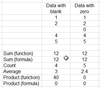
Adding numbers together gives you the same answer for data with blanks or zeros, using sum() or using a cell formula.

The count() function counts the number of non-blank cells - four for the first data set, and five for the second.

The average() function also knows to skip blanks, so you get an average of 3 for the data with a blank (because 12/4 is 3), and 2.4 for the data with a zero (because 12/5 is 2.4).

However, things get hinky when you multiply values together. If you use the product() formula Excel knows to skip blanks. The data set with a blank multiplies 1 by 2 by 3 by 4 by 5 and gives us a product of 40, whereas the data with a zero includes the 0 in the product and gives us (correctly) a product of 0. If you use a cell formula instead, Excel treats the blank as a 0, and gives you a 0 product for both of the data sets.

So, we will need to be careful when we are dealing with a data set with a mix of blanks and 0's to make sure that we're getting the right answer. As a general rule, using Excel's built-in functions will give you better results because they properly ignore missing values, so make a habit of using Excel's functions.

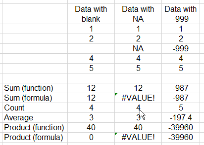
One other thing - if you are working with other people's data, always make sure you are aware of how missing values are coded in the data set. Sometimes they are represented by blanks. Sometimes they are represented with a text string, like NA. Sometimes they are indicated by a specific code that is an impossible number for the variable, like -999. You can see the consequences of using an NA or a -999 to indicate a blank in Excel in this example - again, the functions still work properly if we use a text label like NA, but cell formulas that try to do math on a text value give an error (#VALUE means that you tried to do an operation on the wrong data type).

And, of course, Excel has no way to know that -999 is supposed to be a blank, so all of the calculations get thrown off. If you're working with data that uses something other than blanks to indicate a missing value, you'll need to do a search and replace to convert them all to blanks.

Okay, so obviously we will need to be on our toes. You'll see that some of the steps in the calculations below are necessary to make sure that the blanks aren't screwing us up.

And...

**Before we go to the next step, let's make a couple of changes that will make the rest of the activity easier**

First, double-click the tab for the worksheet that the PivotTable is in (which should say Sheet1) and change it to Pivot.

Second, select "File" → "Options", and then switch to the "Formulas" settings in the "Excel Options" window. Find the option that says "Use GetPivotData function for PivotTable references" and un-check it. This will make it possible to build our spreadsheet formulas by clicking into PivotTable cells.

Third, select the first value in the "Average of Occupancy" column for 1999, which should be B6. Find and select the "View" tab, and click "Freeze panes", then select "Freeze panes" from the list - this will divide the window into column and row labels that do not move as you scroll, which will help you keep track of what each column total is for. You should be able to scroll down to the bottom of the table and see the occupancy rates in the Grand Total row for each of the years, like so:

Occupancy sums

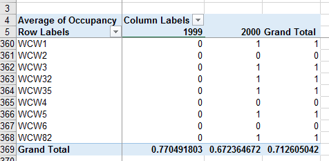
3. Occupancy rate: Excel has the annoying habit of calling everything a "Grand Total" even if something else other than a sum is selected - so, even though the labeling is a little unhelpful, the Grand Total row actually has the averages for each year, which are the occupancy rates. Copy the 1999 rate from B369, switch to sheet "Estimates", and paste-special as values to cell C2. Do the same for the 2000 estimate - copy from Pivot sheet C369 and paste-special in cell C9 of the Estimates sheet.

To calculate the 95% confidence interval, we will use Wald CI's (which, you may remember, can be a problem with values close to 0 or 1, and with small sample sizes, but neither of those issues is a problem here).

Standard deviation of the occupancy rate: The standard deviation of a proportion is the square root of p(1-p). In cell D2 use the formula =sqrt(c2*(1-c2)) to calculate the standard deviation of occupancy rate for 1999. Copy and paste this formula to cell D9 to get the standard deviation for 2000.

Sample size: To get the sample sizes you need to change the pivot table from displaying averages of Occupancy to displaying Counts. You'll see there were 244 nests observed in 1999, and 351 in 2000 - enter these in the n column of Estimates (E2 and E9, respectively).

Standard error: The standard error of a proportion is the standard deviation divided by the square root of the sample size minus 1 (that is, sqrt(sample size - 1)) - make it so (you should get a value of 0.026976 for 1999, and 0.025088 for 2000).

Uncertainty: The uncertainty used to calculate confidence intervals is...problematic for proportions. The method we have been using of calculating an uncertainty value and then adding it and subtracting it from the estimate is called the Wald method, and we already know how that's done. Using Wald confidence intervals with proportions is okay if you have a large sample size (which we do), so that is what we will do now. But, bear in mind that with small sample sizes they can be inaccurate, the the point that they can give impossible values, such as upper limits above 1 or lower limits below 0. Our sample sizes are large enough, and our estimates are far enough from 0 and 1, to use the Wald method accurately, so in cell G2 type =1.96*F2 to get your uncertainty value (which will be 0.052873). Copy and paste this to F9 for 2000 (it will be 0.049172).

What if we had a smaller sample size? We would either need to use an adjustment to the Wald method that allows for asymmetry in the interval, transform the data to a scale that isn't bounded (like calculating the log odds) for confidence interval calculation and then back-transforming to the original data scale, or use something like profile likelihood confidence intervals that can't exceed 0 and 1. None of these are needed here, but if you're interested let me know and I'll be happy to walk you through the process.

Confidence interval lower and upper limits: The lower limit and upper limit are just the estimate minus or plus the uncertainty, respectively. Calculate these values in H2 and i2, and then copy and paste the cells to H9 and i9.

4. Initiation rate is also a proportion of territories that were occupied at the beginning of the season that initiated breeding, for the territories that were occupied. To get this we need to average the 0's and 1's from the Initiation column, like we did for Occupancy. Note that there are in fact territories that have a 1 for initiation but a blank for occupancy, because the territory was found after breeding had started. We could have entered a 1 for occupancy for those territories because it's logical to assume that a territory that initiated breeding had to have been occupied, but since the presence of birds at a nest is extremely helpful in finding the nest it was much more likely that we would find a territory later in the season if there were ravens using it. To avoid biasing our occupancy rates we did not back-fill the occupancy column when we found new territories after they had initiated breeding.

In your Pivot tab, drag Occupancy from the VALUES to the FILTERS
Drag Initiation into the VALUES, and set it to calculate an Average
You will now see Occupancy in the first row, above the PivotTable, with a drop-down list that says (All). Drop down the list and click on the 1 - this will take out any of the nests that were not known to be occupied before they were found.

Initiation rate is calculated the same way as occupancy rate - the average of the 0's and 1's is the same as a count of the total number of territories that initiated breeding divided by the total number of territories that had been found to be occupied. You can copy and paste-special the estimates to the Estimates sheet. Then switch from Average to Count and enter the sample sizes in the n column for the initiation rates.

The calculations are the same for initiation as for occupancy, so you can copy/paste the formulas for standard deviation, SE, uncertainty, and the lower and upper CI bounds from the Occupancy rows to the Initiation rows. If all goes well you'll see:

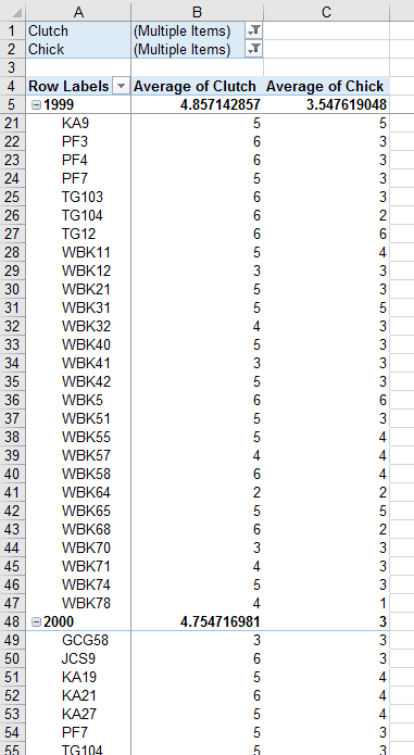
5. Clutch size. Average clutch size is easy - we just need to take an average and standard deviation of the data. All of the blank rows will be omitted automatically.

Drag the initiation variables out of Σ values. You can leave Occupancy in as a filter, because all of the nests with clutch size information are occupied.
Drag Clutch into Σ values and set it to take an average.
Drag Clutch into Σ values again and set it to standard deviation.
Drag Clutch into Σ values a third time and set it to count.
Copy the averages, standard deviations, and sample sizes (counts) from the PivotTable's subtotals for each year and paste-special as values in the Estimates sheet.
Calculate the standard errors - the formula is a little different, so it isn't copy/paste-able from the proportions... this time divide the standard deviation by the square root of sample size (not sample size minus one).
Calculate the uncertainty - this is the critical t-value multiplied by the standard error. If you recall from the stat review, we get a critical t-value with the tinv() function. The formula for the uncertainty for 1999 will go into cell G4, and is =tinv(0.05, E4-1)*F4. This is copy/paste-able to the 2000 estimate.
The confidence interval is the mean clutch size ± uncertainty - make it so.

6. Hatching success is the proportion of eggs that hatch. We could get this in three different ways:

We could divide the average number of chicks by the average number of eggs.
We could divide the number of eggs by the number of chicks for each nest, and then average these.
We could sum up the total number of chicks and divide by the total number of eggs.

We'll try all three and see if they agree.

Drag the Clutch standard deviations and counts out of Σ values, but leave the average there - since there is only one record for each nest using the Average doesn't change the data in the table (because the average of a single value is the single value), but the "Grand total" row becomes a (poorly labeled) average of the values in the table.
Drag Clutch into the Filters.
Drag Chick into Σ values and set it to an average (again, the values in the table are still just the single values, but the Grand total at the bottom is now the average number of chicks).
Drag Chick into the Filters.
For the Chick filters, select everything except blank (click on "Select multiple items" and then un-check the blanks).
For the Clutch filters, select everything except blank (same thing - un-check the blanks).
Drag Year out of the columns and into the rows, before Nest.ID

Your table should now look like this (note that the first row of the table showing is row 21, because I scrolled down so you can see the 1999 and 2000 labels):

Now we will calculate the chicks per egg for each nest - this we have to do outside of the PivotTable:

In cell D4 enter "Chicks/egg", and in D6 enter =c6/b6 - this divides the number of chicks by the number of eggs.
Copy and paste this to the rest of the cells, skipping the mean for 2000 row (row 48).

Now we will lay out a table for our results (we don't want this over-written when we change the PivotTable layout, so we'll put it well off to the side):

In cell o6 enter the label "Method", and in P6 enter the label "1999", and in Q6 enter "2000"
In cell o7 enter "Average chick/egg", in o8 enter "Average chick/Average egg", and in o9 enter "Total chick/total egg"

The calculation for the firs two can be done with the current table, so:

In cell P7 enter =average(d6:d47) - this will give you the average of the chicks/egg you calculated in column D for the 1999 data.
In cell Q7 enter = average(d49:d101) - this does the same calculation but for the 2000 data.
In cell P8 enter =c5/b5 - this is the average of the chick data divided by the average of the egg data for 1999.
In cell Q8 enter =c48/b48 - same calculation but for 2000.

If all went well your table looks like this:

If so then select all the cells, copy, and paste-special as values - we will need to change the PivotTable for our last calculation, and don't want these to change too.

For our last method we need to change the averages to sums for both chick and egg, and then divide total chicks by total eggs:

Change the field settings for both variable to Sum in the VALUES box.
In cell P9 enter =C5/B5 - this is the total chicks divided by the total eggs in 1999
Do the same calculation in Q9 for 2000

If all went well you'll see that mean chicks/mean eggs and total chicks/total eggs are both the same. If that's what you got, copy and paste special values so that these don't change as we change the PivotTable in the next step.

But, we have an issue, because average of chicks/egg is different, so which should we use?

Fortunately, there is a right and wrong way to do this calculation (or rather, a right way and two wrong ways). What we actually want to know is the average chicks/egg, which in statistical terminology is the "expected value" of a ratio of two random variables. Expected value is another way in statistics to say "mean" (which is another way to say average). The mean of the ratio of two random variables, like chicks/egg, is the same as the mean of the first variable divided by the mean of the second only if the two variables are not correlated with one another. It would be truly surprising if the number of chicks in a nest was completely uncorrelated with the number of eggs laid, so we shouldn't expect the mean number of chicks divided by the mean number of eggs to be an accurate estimate of hatching success. Given that, the only correct value of the three is the mean of the number of chicks divided by the number of eggs in each nest - the values in column R.

If we didn't account for this, and used one of the other methods, what would happen? We could correct the other two methods by subtracting the covariance between the number of chicks and the number of eggs - covariance is like a correlation that doesn't fall between -1 and 1 (in fact, correlation is covariance divided by the product of the standard deviations of the variables, which is constrains a correlation coefficient to fall between -1 and 1). If we don't subtract the covariance between the chicks and eggs, given that we expect the covariance to always be positive (i.e. more eggs means more chicks) we would consistently over-estimate hatching success. But, since the amount of covariance can be different in different years, the amount of bias wouldn't be consistent between years, and we may end up with years that seem either to be more different or more similar to one another than they actually are if we don't properly account for this effect.

So, now that we know which calculation is correct, copy and paste the averages of chicks/egg to your Estimates sheet.

To calculate the standard deviations, in the Estimates sheet select cell D5, enter an =stdev( and without hitting ENTER switch to the Pivot sheet and select the range of values for 1999 in column D (they are in D6 to D47). This should give you a value of 0.2240. Repeat the calculation for 2000, using the Pivot data in D49 to D101 (you should get a standard deviation of 0.2280).

Finally, we need a sample size - if you select the rows for the 1999 chicks/egg in Pivot the count of cells selected will show up in the status bar at the bottom of the worksheet - you'll see there are 41 nests from 1999 that had eggs. If you do this for 2000 as well you'll see there were 53 nests with eggs. Enter these as your sample sizes.

You can now copy and paste special the values for the estimates, the standard deviations, and the samples sizes to your Estimates sheet for hatching success. The standard errors, uncertainties, and confidence limits should all be copy/paste-able from the average clutch size row.

7. The proportion of nests that fledge will be a count of all the nests that have one or more chicks fledged divided by the number of nests with fledging data. Keep the PivotTable in its current layout, with Year as row labels.

You can delete column D now that we have the calculations of chicks/egg done - it will get over-written by the PivotTable as soon as we start changing things.

We need a count of the number of cells that have non-zero numbers of chicks fledged - we'll have to get these with two different PivotTable layouts. The first will give us the number of nests with at least one chick fledged.

Take chicks and clutch out of the filters and Σ values.
Drag Fledge into the VALUES (as a count) and then again into the FILTERS - Excel seems to assume you made a mistake if you drag a variable into both the filters and values box, so when you do the second drag of Fledge into values you might then have to drag it into filters again. Be persistent, show Excel who's boss.
Drag Year into the COLUMNS (take it out of the ROWS)
Drop down Fledge in the Filters above your table, select multiple, and un-check blank and 0.

Your table should now show nests that had at least one chick fledged, and the column Grand Total is the count of these nests. We'll calculate the values in the Pivot sheet:

Enter the label "1999" in cell o14 and enter the count for 1999 in P14 (it should be 69)
Enter the label "2000" in cell o15, and enter the count for 2000 in P15 (it is also 69)
In P13 enter the label "Fledged 1 or more".

Now, drop down the Fledge filter again and check the 0 - the count now includes all of the nests, including those that didn't fledge chicks. Enter the label "Total" in Q13, and enter the totals for each year in Q14 and Q15 (they are 104 and 147, respectively).

Now to calculate the rates:

Label cell R13 "Prop fledged"
In cell R14 enter =p14/q14
Copy and paste this to R15

You should get rates of 0.663462 for 1999 and 0.469388 for 2000. If so, copy these and paste-special to the Estimates sheet for "Proportions of nests that fledge".

The sample size is equal to the total number of nests, in column i, so you can enter those in your Estimates sheet as well.

These are simple proportions, so you can copy/paste the formulas from occupancy rate for the standard deviation, SE, uncertainty, and confidence limits.

8. To calculate the average number of chicks fledged per occupied nest, we just need to use the fledging data for nests with Occupancy = 1.

Keep Year as a row label
Keep Fledge as the VALUES, and set it to Average (we won't use the average from the table because it will be wrong, but we'll use this to see that it's wrong).
Drag Fledge out of the Filters, and drag Occupancy in
Set the Occupancy filter to only show 1

The table should look like this (scrolled to show the start of the 2000 data:

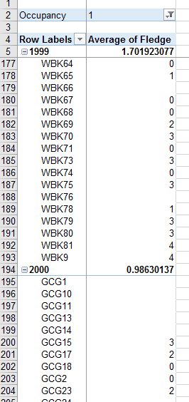
It seems like we have what we want, but we don't yet because of the blanks - we didn't enter 0's into the Fledge column for territories that were found after eggs or chicks were already in the nest, because we didn't want to bias our occupancy rate data. But here we are safe in knowing that an occupied nest that never fledged chicks should get a value of fledged of 0, so we should set those blanks to a value of zero for this calculation.

Select any data cell in the PivotTable and select "PivotTable Options" from the menu that pops up.
In the "Layout and format" tab find "For empty cells show:" and enter a 0
Click OK

You should now have 0's where there were blanks. But...the averages didn't update to use those 0's.

So, we can't use the averages that the PivotTable calculated. But, if we use the data in cell formulas outside of the PivotTable the 0's get used as 0's, and we'll get the right values.

In cell C4 enter "Mean fledged".
In cell C5 enter =average(b6:b193) - you should get 0.9414... as the average. This is different from the PivotTable value because it is (correctly) using the zeros.
Repeat for 2000 in C194 (you can copy/paste the formula but the make sure you update the rows to include all the 2000 nests).
We can get the standard deviations and sample sizes while we're at it - enter StDev in D4, and n in E4. Then, in D5 enter =stdev(b3:b193), then in E5 enter =count(b3:b193)
Repeat the calculations for 2000 - again, you can copy/paste, but then be sure to update the rows.

Once you have these done you can copy/paste-special values the estimates, standard deviations, and sample sizes to your Estimates sheet. The SE, uncertainty, and confidence limits formulas can be copy/pasted from the average clutch size row.

9. Last, to calculate the number fledged from initiated nests, pull Occupancy out of the filter and put in Initiation, and set the filter to only nests that initiated (1).

The formulas you used to calculate chicks fledged per occupied nest updated, but the cell references are wrong, since there are fewer initiated nests. Adjust the cell references for the means and standard deviations, and enter the new sample sizes (the Count of Initiation subtotals for 1999 and 2000). Copy the mean, sd, and n for each year and paste-special as values to the Estimates sheet.

Your final table will look like this:

10. Time to do some graphing - we have a lot of stuff to look at in the Estimates table, but it's hard to tell how different the values are between years in a big table like that.

Let's start with a chart of the estimates that are proportions, for 1999.

Select the labels for occupancy rate, initiation rate, hatching success, and proportion of nests that fledge, and then select all the estimates next to them for 1999 - you can hold down the CTRL key and click on each one of these to select them (they are not sitting right next to each other, so you'll need to use CTRL to get them all without including clutch size)
Select the "Insert" tab, and then insert a column chart, . Select the first option 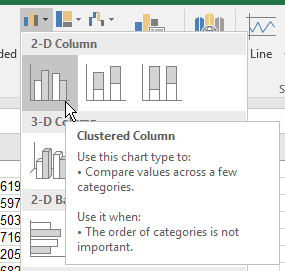for the column chart type.
Now we're going to add the 2000 data - right-click on the bars in the graph, and select "Select data".

In the "Select Data Source" window, click on "Add" to add a new "Legend Entries (Series).
For the series name, click on A9, which has the year 2000 in it. For the "Series values" click the zoom box, , and then click each of the 2000 statistics (in cells C9, C10, C12, and C13) and click OK. It isn't necessary to select the names of the statistics again, they will be used from the other series.
Before you finish, click on Series1 and click "Edit" - select the cell with 1999 in it to be the series name. Click OK to record the change.
Click OK again to finish selecting the new data series.

Now we want to add the legend to tell us which year is which. Select the graph, and click on the + to get the "Chart Elements" dialog, and check the box next to "Legend" - you now have the years identified.
We took the trouble to calculate confidence intervals, so we should use them:

Click on one of the 1999 bars, and click on the options + and then for "Error bars" click on the right arrow and select "More options".
Check the box for "Custom", and then click the "Specify value" button.
For the positive error value, click the zoom box and select the uncertainties for the 1999 statistics you're plotting (in cells G2, G3, G5, and G6). Do the same for the negative error values.

Now, click on one of the 2000 bars to select the series, and add error bars for those the same way.

Change the chart title to "Reproductive rates that are proportions"

Now try making a chart for the three statistics that aren't proportions - average clutch size, fledged per occupied nest, and fledged per initiated nest. You can title it "Reproductive rates that are averages".

You can see that there are some differences - the reproductive rates are listed in your table in a chronological order - the birds have to occupy a territory, then initiate breeding, then lay eggs, then hatch the eggs, and finally fledge chicks to reproduce for the season. As you work from left to right on the graph you'll see that the values tend to go down. Getting all the way through to the end of the season and having successful reproduction is not so easy.

Also think about how these numbers might tell you something different about conditions for the ravens. There are a couple of reasons why occupancy rates might be low - the conditions may be poor for reproduction (either in terms of food available in Feb/Mar when the ravens are deciding whether to attempt breeding or not), or alternatively it could be the population crashed the previous fall and winter, and there are fewer individuals to occupy territories. If it's the former, then all the reproductive measures for the rest of the season may be low - a bad year for occupancy may be a bad year for laying eggs, hatching chicks, and raising them to fledging. But, if it's the latter, then the birds that are around to breed may have lots to eat, and may do really well - low occupancy followed by high clutch size, hatching success, and fledging could indicate that there is a density-dependent increase in those values. We would also expect that clutch size should be primarily a function of the mother's body condition, but fledging success depends on the ability of the parents to provision food, and on the nest predation rates in the area. Calculating these different variables is not just alternative ways of calculating the same thing, comparisons between them can give you some insight into what factors might be affecting their reproduction.

That's it! Save your worksheet for the final demographic monitoring write-up.