Lab 17 - Apparent survival estimation in demographically open populations

We're going to make one more visit to the wonderful world of mark/recapture data to learn about survival estimation. The data will look familiar, as we will be using capture histories, but the design of the study, the characteristics of the populations, and the way we model the capture histories will all be different. The survival analysis we will be working with is called the Cormack-Jolly-Seber model, named for the people who developed the approach.

One thing that should be obvious is that you can't simultaneously assume demographic closure and estimate survival, since deaths violate the demographic closure assumption. By definition, survival analysis doesn't assume demographic closure. Less obviously, we can also partially relax the geographic closure assumption - we are going to be working only with re-captures of animals that were captured and marked in the first capture period, so movement into the population is irrelevant (the immigrants will not be marked, and can't affect our analysis). Emigration out of the population is still an issue, however, because marked individuals who leave the population can't be recaptured, and will appear to have died. Since this is a possibility, as long as we can't be certain the population is geographically closed we refer to these survival estimates as apparent survival, since some of what appears to be mortality may actually be emigration.

Relaxing closure assumptions is a big change, because they had important consequences for our interpretation of the zeros in our capture histories. If a population is demographically and geographically closed we could treat zeros in our capture histories as known outcomes - a zero was assumed to be an animal that was alive and present in the population but went undetected. It didn't matter whether the zeros were leading or trailing - a leading zero (such as 011) meant we missed capturing the animal in the first trapping period, and a trailing zero (110) meant we missed recapturing the animal.

Since we are no longer assuming demographic closure, trailing zeros could potentially be due to two different events: 1) the animal survived but went undetected, or 2) the animal died. We will not be using "dead recoveries" - that is, deaths are not detected, so there's no way to tell a mortality from a failure to encounter a living animal. Our survival models will have to account for this ambiguity.

In addition to having to treat trailing zeros differently, we will need to change how we interpret the entire capture history when we estimate survival. As before, we will call the encounter probability p. However, now we are primarily interested in what happens in the intervals between captures, because those are the periods of time over which survival or mortality are occurring, so we will model the probabilities of survival between the captures. Survival probability is symbolized with a Greek upper-case phi, or ϕ. To begin, we'll assume that p and ϕ did not change over time, so a single p and ϕ are used for all time periods.

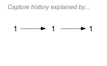	To the left is the simplest capture history to model, which is 111. With survival estimation, all capture histories begin with a capture - the capture history begins when an animal is marked and released for the first time. There is no capture probability assigned to the first capture (we'll call this time 0, or t=0) because having a first capture is a given (if we were to assign it a probability, it would be 1, because we know we caught the animal at t=0). If you click on the image it will change to show the only possible explanation for this history. In order for the animal to be captured the next time it has to survive until the second capture period with probability of ϕ, and then be captured again with a probability of p. The probability of both surviving from t=0 to t=1 and being captured at t=1 is ϕp. Likewise, to be detected at t=2 the animal needs to survive another year and be captured again, which also has a probability of ϕp. We calculate the probability of the entire history by multiplying the probabilities along the path defined by the arrows - the probability of surviving and being captured at time 1 and surviving and being captured at time 2 is ϕpϕp.
Note that although the capture history looks just like the kind we would use to estimate population size, the sampling design is different. We don't need to keep the captures close together in time because we don't want to assume demographic closure - the captures are spaced far enough apart that some mortality is likely to have occurred, and usually the captures are over ecologically meaningful time periods, such as seasons or years. We'll be working with data collected each year, so ϕ is annual survival probability, and p is the probability of being detected in a given year.
	Now, let's look at a history with a 0 in it. If you click once to see the model, you'll notice that the only difference from our model for 111 is that we used (1-p) to model the 0 at t=1. An embedded zero (i.e. zeros followed by ones) like this one is not ambiguous - since we know the animal was alive at time 2 it must have been alive at time 1 as well (so, we are assuming animals aren't dying and coming back to life - the "no zombie apocalypse" assumption, or NZA). The probability of this capture, then, is ϕ(1-p)ϕp
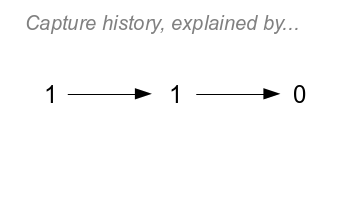	The NZA assumption can't be invoked with a trailing zero though. Things are clear enough for the first recapture - the animal has to have survived with probability ϕ to have been recaptured at time t=1, and the probability of that capture is p. But, for the second period there are two possibilities - click once to see the first: Option 1 is that the animal could have died between t=1 and t=2, with a probability of 1-ϕ. We aren't including dead recoveries, so if an animal dies then there is no chance it will be recaptured, and we don't need to include a probability of recapture along that path. The probability for this option is ϕp(1-ϕ) Click again and you'll see the second possibility (Option 2) - the animal could have survived with probability ϕ and then gone undetected at t=2 with probability 1-p. The probability for this option is ϕpϕ(1-p) The two possible fates for the animal at time 2 are mutually exclusive alternatives - that is, an animal can't both be alive and dead at the same time (NZA). We can thus add the probabilities for each path to give us the probability of capture history. This is the addition rule for mutually exclusive "or" probabilities, if you remember your intro stats. So, the probability for the whole history is: ϕpϕ(1-p) + ϕp(1-ϕ) If you click on the image one more time you'll see the branching paths that represent both of these possibilities - the probability of each path is the product of the coefficients along each step of the path, and the sum of the two paths is the probability of the history.
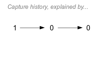	The last possible history, 100, is the most complicated because it has two trailing zeros. If you click on the image once you'll see the first possible explanation for the history: Option 1 is that the animal died before the first recapture at t=1, with probability 1-ϕ. Click again to see the second possible explanation (Option 2) - it's possible that the animal survived undetected to the first recapture and then died before the second. The probability of this option is ϕ(1-p)(1-ϕ). Click again to see the third possible explanation (Option 3) - the animal could have survived undetected through both recaptures. The probability of this option is ϕ(1-p)ϕ(1-p). Since any of these three possibilities may have occurred, and they are mutually exclusive, we add them up to get the probability of the capture history: (1-ϕ) + ϕ(1-p)(1-ϕ) + ϕ(1-p)ϕ(1-p) Click once more to see the full set of pathways possible, but just like with history 110 you can find the probability of the history by multiplying coefficients along each path and then adding them together across the three possible paths through the diagram.

It's possible to algebraically simplify these formulas - for example, for history 110 we could express the probability ϕpϕ(1-p) + ϕp(1-ϕ) as ϕp - (ϕp)². The simplified version is easier to enter into Excel, but it is less clearly a model for the 110 capture history. We will stick with the un-simplified versions to help us understand how the formulas are related to the capture histories.

To keep things simple today we won't allow new animals to be added to the population in the second capture period, so we won't have 010, 011 capture histories. If we were going to use these we would ignore the leading 0 and model the histories just using the survival and capture probabilities for the t=1 to t=2 periods. Adding new animals to a study is common when the recaptures at t=1 and t=2 were actual captures - capturing a previously unmarked individual and just letting it go would be a pretty foolish waste of effort (note that adding new captures in the last period would tell us nothing about survival, so there would never be a need for a 001 history). But, if we initially captured animals, marked them conspicuously, and then resighted them later rather than capturing them again, we would only have histories with 1 in the first position - we will just work with animals that were all marked at time t=0.

Time-varying encounter and survival

The probabilities of capture histories above all use a single p and a single ϕ, which means they assume encounter and survival probability to be the same for each interval - we can call this model ϕp. It is quite possible that survival and encounter probabilities are not constant, and we could allow one or the other, or both, to change over time. A model in which encounter probability changes over time but survival is constant would be called model ϕp_t, and the capture histories would have these probabilities:

Table 1. Model ϕp_t capture history probabilities

A single ϕ is used, but the encounter probabilities are subscripted to indicate the capture period, and we use p₁ for t=1, and p₂ for t=2.

If survival varies but encounter probability does not then we would have model ϕ_tp. The capture histories would have the probabilities:

Table 2. Model ϕ_tp probabilities.

Finally, it's possible that both encounter probability and survival vary over time, which gives us model ϕ_tp_t. The probabilities for this model are:

Table 3. Model ϕ_tp_t probabilities.

We can use AICc to tell us which of these models best describes our data.

Estimating survival

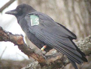
We will return to the ravens of the West Mojave for this exercise. In addition to studying their breeding biology, my colleagues trapped and marked a large number of ravens at the landfill at Edwards Air Force Base in 1996. Birds were either equipped with a radio transmitter backpack and wing tagged, or were just given wing tags (the picture on the left gives you an idea of what the wing tags look like, although this is a picture of a crow...I couldn't find a good wing tagged raven picture for you, sorry). The data we actually collected in this study is a little complicated for this class - we had a mix of live and dead recoveries, had detection periods in both the summer and winter, distinguished between adults and juveniles, and there were several trapping events in which new birds were added to the marked population.

We will work with two simplified versions of the data, one with only three years that you will use to try out defining the models for the capture histories, and one with all five years of data for the birds caught in 1996 that you can use to fit all four of the models we're interested in and compare them with AICc.

First, open this Excel file. You'll see that there are two sheets, one called Example and one called Data. In both I have already summarized the capture histories for you. We will start with Example, which has only three years of data and has encounter history probabilities that are not too complicated to work with.

1. Set up the Example worksheet for ML estimation. I have given you a column of labels for the four parameters (D), and a place where you can enter your link functions and betas (E and F). You also have a column for the multinomial capture histories (H), and a label for the log likelihood (cell C10).

In cell E2 enter the sine link function - type =(sin(f2)+1)/2. Copy and paste this function to the rest of the MLE cells.

We will ultimately want to fit models that either have time-varying survival, capture probability, or both. To make that simple you will set up your multinomial probabilities in column H as though both survival and capture probabilities are time varying. To fit models that have constant survival or capture probabilities, like model phi,p, we will enter a beta for phi1 and p1, and then make phi2 and p2 point to their values - we will only let Solver vary the betas that are entered as numbers, and the others will use the same values.

So, to make this work:

• Type a 0 in cell F2 and F4. This will set the initial beta to 0 for both phi1 and for p1. We are starting them both at the same place, but we will have Solver change these two cells, so we will end up with a different estimate of p1 and phi1.
• In cell F3 type =f2. This sets the beta for p2 to be the same as for p1 - whatever value Solver picks for p1 will also be used for p2...this model thus uses a single, constant p.
• In cell F5 type =f4. This sets the beta for phi2 to be the same as for phi1. Like with the capture probabilities, phi1 and phi2 will now be the same, which means this first model uses a constant phi.

Under the "Multinomial probability" label in column H you will enter your probabilities for each capture history. This is where we translate the equations in Table 1 above into cell formulas in the spreadsheet. Take a crack at doing this yourself - use the MLE's as phi and p, not the betas. Even though we have set p2 to be the same as p1, and phi2 to be the same as phi1, lay out your multinomial probabilities using the p1, p2, phi1, and phi2 MLE's that match the formulas in Table 1 - this will allow us to specify a different model just by changing the betas. If you get it right, the multinomial probabilities sum to 1. I'll give you the hardest one, for history 100 - its formula is:

(1-ϕ₁) + ϕ₁(1-p₁)(1-ϕ₂) + ϕ₁(1-p₁)ϕ₂(1-p₂)

To translate this into an Excel formula, enter into cell H5:

=(1-E2)+E2*(1-E4)*(1-E3)+E2*(1-E4)*E3*(1-E5)

You should get a value of 0.6875 for the multinomial probability of this history.

The rest are easier (shorter, at least), so try them out yourself... the formulas are:

History 111 (cell H2): ϕ₁p₁ϕ₂p₂

History 110 (cell H3): ϕ₁p₁ϕ₂(1-p₂) + ϕ₁p₁(1-ϕ₂)

History 101 (cell H4): ϕ₁(1-p₁)ϕ₂p₂

When your done, your table should look like this:

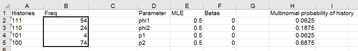
Note that you can't see in this screenshot that the beta for phi2 and p2 are both formulas pointing to the cells above them, but make sure you have the number 0 entered for phi1 and p1, and formulas for phi2 and p2.

If this is not what you're getting, check your formulas - check that you used parentheses where they were needed.

Once your probabilities are all correct, beneath the "LnLikelihood" label in cell C10 we will calculate the log of the likelihood function. In C11 sum the frequencies multiplied by the logs of the probabilities. We did this in our population estimation sheet a couple of weeks ago, you can do it with an array formula in this cell (hint: it's =sum(freqs*ln(probs)), just replace freqs and probs with the correct cell ranges). If you do it right you'll get a value of -228.71. We don't need to calculate a multinomial coefficent (the gammaln() function) because we aren't estimating the frequency of animals that were never caught this time - all we need is the "probability part" of the multinomial likelihood.

You're ready to roll! Time to get some estimates.

2. Start up Solver, and get your estimates for phi and p. Start up Solver, and set cell C11 to maximize, by changing JUST the betas in f2 and f4 (the betas in f3 and f4 will update automatically, don't vary them). Your results should look like this:

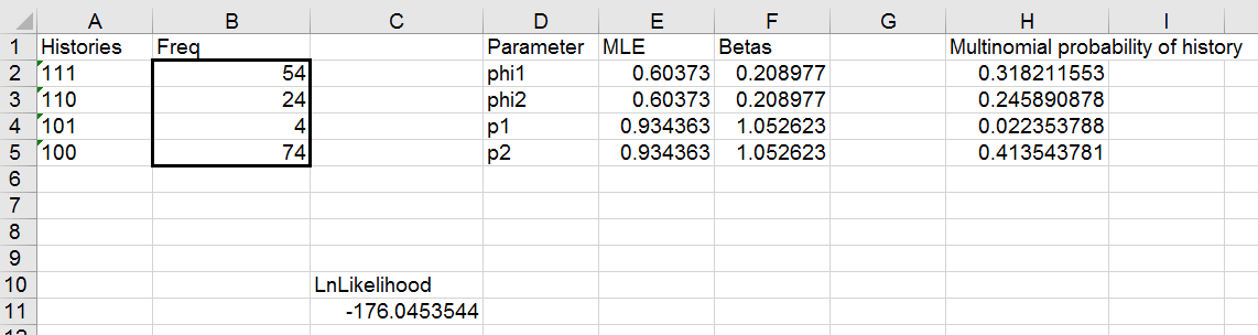
You should see that even though we have a line for phi1 and another for phi2 there is just one estimate for phi, because the beta for phi2 is just a pointer to the beta for phi1. Same goes for the p's - even though there are lines for p1 and p2 there is only one value that is being used for both.

Now, to get estimates for the model with time-varying survival but constant capture probability we would just need to:

• Copy the beta from F2 and paste it into F3 - F3 is no longer a formula pointing to the value in F2, it is its own separate value.
• Start Solver, and have it maximize the log likelihood by varying the betas in F2, F3, and f4. This will produce a separate estimate of phi1 and phi2, but only a single estimate for p because p2 is still just a pointer to p1.

Run this model, and you'll get results that look like this:

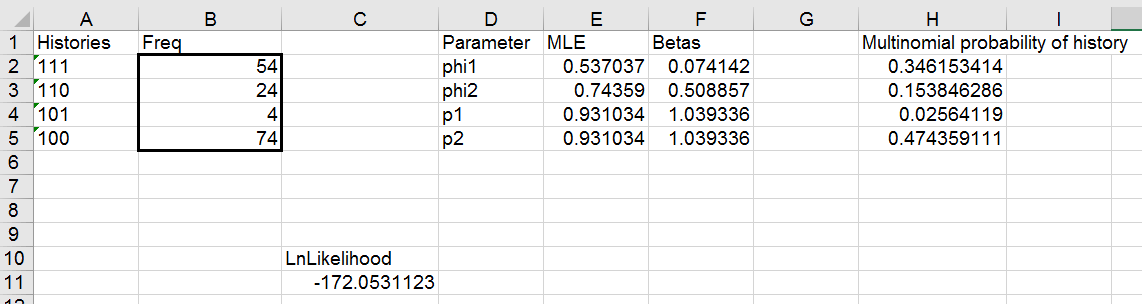
With this model we have a difference in survival for the two different time periods between captures. The log likelihood is higher for this model, but we used an additional parameter to achieve that increase in log likelihood, so we would need to do some model comparison using AICc to tell which is better supported by the data. We'll save that step for the full data set, which we will turn to now.

We won't make an AIC table for the Example data set, but the graphs below let you compare observed and expected numbers for the three models you fit, plus the problematic model with time-varying survival and time-varying encounter probability:

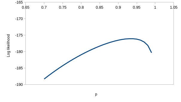
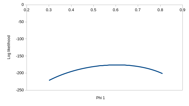
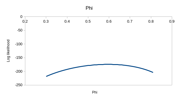
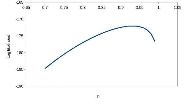
Finding the maximum likelihood values for p and ϕ isn't hard for the simplest model, ϕ.p. in the upper left - you'll see that values around 0.6 for survival and 0.9 for detection probability produce the highest likelihood.

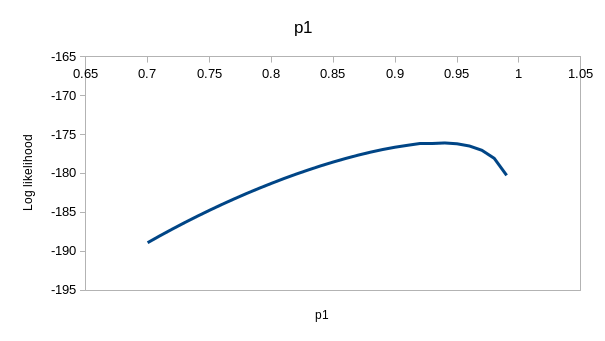
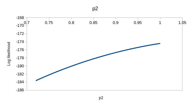
Similarly, with the second model in the upper right, with constant survival but time-varying detection probability (ϕ.p_t) - values of 0.6 or so for ϕ and 0.9 and 1 for the detection probabilities work well. The observed bars can get closer to the expected with two different probabilities of detection than with one, but the match between observed and expected is not perfect with the ϕ.p_t model.

With just three years of data we run into trouble with the last two models, because it is possible to make the expected values exactly match the observed values for both of them. 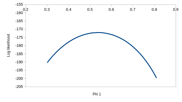This is a problem when the number of parameters estimated by the model is equal to or greater than the degrees of freedom available - with four capture histories we have four different capture histories, which means we have 4-1 = 3 degrees of freedom, so a model that has 3 parameters consumes all of them and explains the data perfectly. 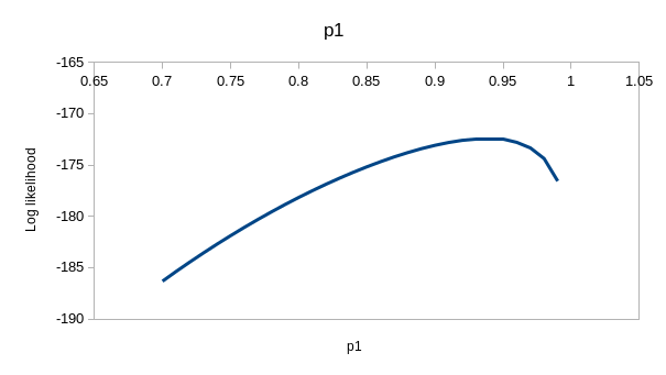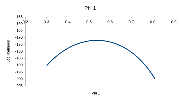If you enter the values for model ϕ_tp of 0.537 for the first ϕ, 0.743 for the second, and 0.931 for p you'll see that the observed and expected values are virtually identical - this model is explaining nearly all the variation in the data. If you hover over the "(profile at ML)" links you'll see the likelihood function for each of the estimates, which we could use to get confidence intervals - they are all curved around the estimate, so the data has enough information in it to give us good estimates for this model

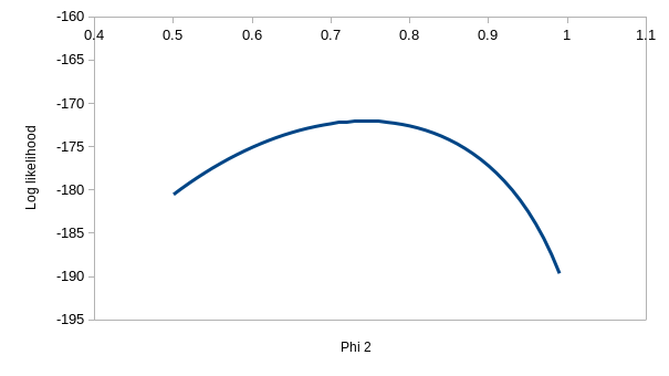
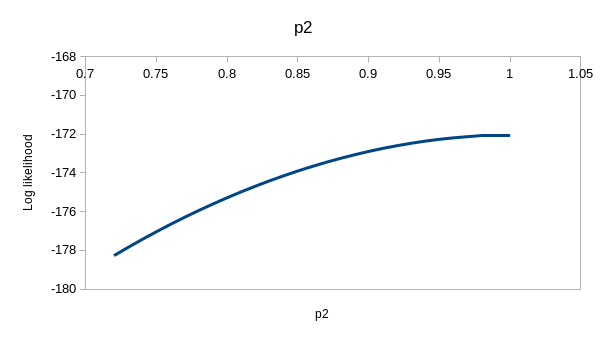
But, we're out of variation to explain with model ϕ_tp, and model ϕ_tp_t has one more parameter in it. If you enter the values of 0.537 for ϕ₁, 0.692 for ϕ₂, 0.931 for p₁, and 1 for p₂ you'll see that it has almost exactly the same log likelihood as model ϕ_tp. Given that the only difference between ϕ_tp and ϕ_tp_t is that we have two different detection probabilities for the latter, you can turn ϕ_tp_t into ϕ_tp. 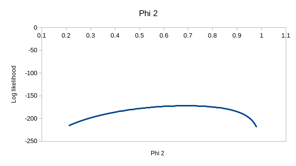by just plugging in the ϕ_tp coefficients into ϕ_tp_t and the log likelihood is unchanged - in other words, if you plug in 0.537 for the first ϕ, 0.743 for the second, and 0.931 for both of the p's you can turn ϕ_tp_t into ϕ_tp, and get the same log likelihood. This means that the ϕ_tp_t model doesn't have a unique, best set of paremeter estimates. You can see the problem with this if you hover over the profiles - the one for ϕ₂ is really flat, which means that a wide range of values could be used and produce a log likelihood that is almost the same.

We won't run into this issue using the full five years of data, because we have a total of 16 possible histories, of which 10 were observed in the study, so we will have plenty of degrees of freedom to fit model ϕ_tp_t. Just bear in mind that although it's possible to use CJS models to estimate survival with as few as three years of data, having only four possible histories limits the models you're able to fit, and adding more years overcomes that problem.

3. Get estimates for model ϕp for the full data set. Now that you see how this process works, switch to the Data sheet and you'll see that you have a very similar setup as in the Example sheet, but with five years of data for ravens caught in 1996. The multinomial probabilities are substantially more complicated, so I did them for you - you will focus on setting the model parameters to make the four models we will compare (model ϕp, model ϕ_tp, model ϕp_t, and model ϕ_tp_t).

Before you start, notice a few things:

• The histories and their frequencies are in columns A and B. Some of the histories that were possible were not observed - I included them in the list and calculated multinomial probabilities for them so that you can see what the complete set looks like. The full set is also needed to make the sum of the capture histories equal 1, which is helpful for checking your work. Since the log likelihood is calculated by multiplying these frequencies by the log of the probabilities of the histories, the histories with frequency of 0 have zero effect on the log likelihood - we could leave these histories out and it would not affect the estimates of phi or p.
• There are now four survival probabilities: phi1, phi2, phi3, and phi4. They represent survival from 1996 to 1997 (phi1), from 1997 to 1998 (phi2), from 1998 to 1999 (phi3) and from 1999 to 2000 (phi4). I've highlighted the survival probabilities in yellow.
• There are four capture probabilities: p1, p2, p3, and p4. They represent the probability of being observed in 1997 (p1), 1998 (p2), 1999 (p3), and 2000 (p4).
• If you look at the betas in column F, only phi1 and p1 have numbers entered at first. All the rest of the phi's point to F2, and all the rest of the p's point to F6. The sheet is thus set up to find the estimates for model ϕp initially.
• The multinomial probabilities are complicated when there are one or more trailing zeros. The most complicated is history 10000, which are birds caught in 1996 and never seen again. The approach is just like you used for the example, but with more zeros and thus more possible paths. If you double-click on the formula in H2 you'll see there are five different calculations that describe possible paths through the data - each either ends with a mortality (a 1-_phi) except for the final one, which ends with a non-detection in the final year of the study. Don't change anything, and hit ENTER.
• Note that to help me assemble these properly I defined names for each of the values in column E and used them in the formula - _phi1 is just a pointer to E2, _p1 points to E6, and so on. Hit ENTER to get out of edit mode (don't change anything!).

Okay, you can now run Solver to get the estimates - set the log-likelihood to maximize, by changing ONLY cell F2 and F6. If all goes well you'll get estimates that look like this:

4. Record the results for model phi,p. copy the one phi estimate (cell E2) and paste-special its value to the Parameters table - this model is phi,p so paste it into cell B36. Then copy the one estimate for p and paste-special its value into cell B40.

Copy the log-likelihood and paste-special its value to cell B29 - we will calculate an AIC table to compare the four models, and we need the model log likelihoods for this.

Enter the number of parameters (2, a single phi, and a single p) into cell C29.

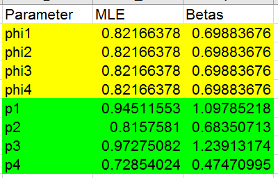
5. Fit model phi_t,p. This next model uses a different value for phi for each of the time periods, but still uses a constant capture probability. To set up this model, all you need to do is change the formulas in cells F3 through F5 to have numeric values rather than formulas. Copy the beta from cell F2 and paste it into cells F3, F4 and F5.

Run Solver again, and this time have it change the betas in F2 through F6 (only F6 needs to change for the p's, the rest are still formulas pointing to this value). If all goes well, you'll get these estimates:

You'll see that, if this model is well supported by the data, there is fairly substantial variation in survival probability between the years. Copy the four MLE estimates for the phi's and paste-special their values to cells C36 through C39. Also copy the single p1 estimate and paste-special its value to C40.

Copy and paste-special the log likelihood to cell B30, and enter the number of parameters into C30, which is... how many? Click here to see.

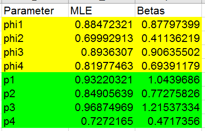
6. Fit model phi,p_t. Now to fit a model with time-varying capture probability, but constant survival, we need to set cells F3, F4 and F5 to point back at the single beta in F2, but replace the formulas in cells F7, F8, and F9 with the value from F6.

• Enter =f2 into cells f3, f4, and f5
• Copy the value from f6 and paste it into cells f7, f8, and f9.

Run Solver again, and this time change cells F2 and cells F6 through F9.  and you should get estimates:

This model predicts low recapture probabilities in 1998 and 2000 rather than low survival in those years.

To record the results, copy and paste-special the single MLE for phi into cell D36, and copy/paste-special the four estimates for p1-p4 into cells D40-43.

Copy/paste-special the log likelihood into cell B31. Count the number of parameters and enter it into C31 (it's the same as the previous model, right?).

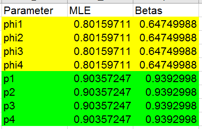
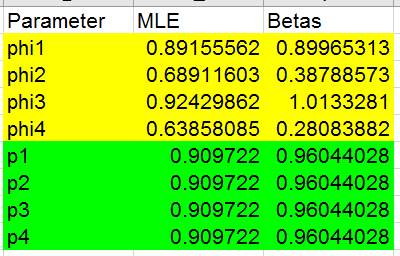
7. Fit model phi_t, p_t. This model will find different betas for every estimate, so copy the beta from F2 and paste it into F3 through F5. Run Solver, and have it change all of the values in F2 through F9. Your results should be:

You'll see that the seemingly lower survival between 1999 and 2000 we saw when recapture probability was held constant is now higher - 0.819 rather than 0.638 - but the recapture probability is lower instead.

Record these results - copy and paste-special the values for all eight of the estimates from column E into cells E36 to E43. Copy/paste-special the log likelihood for this model into cell B32, and enter the number of parameters (which is... what? Count up how many estimated values there were for this model).

8. Look at how the models compare. Now that you have all four of the models we should compare how well the data supports each one.

• In cell D29 calculate the first AIC value - multiply the log-likelihood in cell B29 by -2, multiply the number of parameters in C29 by 2, and add them.
• In cell E29 calculate the AICc - the formula is: =D29 + (2*c29*(c29+1))/(b$19-c29-1)
• Copy and paste the formulas in D20 and E29 to the cells below (C30 through C32).
• Calculate the deltas - in cell F29 subtract the minimum AICc from the first AICc value, using the formula =e29 - min(e$29:e$32)
• Calculate the weights - in cell G29 enter the formula =exp(-0.5*f29)/sum(exp(-0.5*f$29:f$32)) , and enter it as an array formula (CTRL+SHIFT+ENTER)
• Copy and paste cell G29 to cells G30, G31, G32.

You should get a table that looks like this:

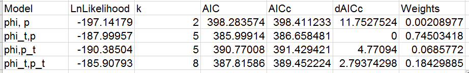
You'll see that there is good evidence that survival is time-varying, since the two models with the best support both allow for varying survival probability. Capture probability may or may not be time varying, since the model with only varying capture probability has substantially less support, but the model with both varying phi and p has moderate support.

If you look at the estimates, the decrease in survival between 1997 and 1998 (phi2) is present in both well-supported models. But, if both recapture and survival probability are allowed to vary over time then survival does not decline substantially between 1999 and 2000 but recapture probability does.

Where could we go from here? There are several things we could do:

• We could try models that have differences in phi or p in some years but not others. Since survival seems to be pretty similar for phi1 and phi3, and for phi2 and phi4, we could make those pairs of values the same by letting Solver vary one and setting the other to equal the parameter being varied. We would have to be careful with this one, though, because fitting models based on patterns found during analysis runs the risk of over-fitting, which can lead us to interpret a model that seems to be well supported but isn't accurate.
• We could see whether there are differences in survival by age class. Ravens are easy to age in their first year, so we could see if there is evidence that first year survival is different. We would need to split the capture histories by age group and see if the animals that were captured in their first year had different probabilities of survival for the first year after capture compared to the other, older birds.
• We could use individual covariates. It is possible to have the probabilities of survival or capture depend on the individual characteristics of the ravens (such as their weight). The setup for this type of analysis is different, so we won't attempt a model like this in Excel, but it is possible to test hypotheses about whether bigger birds survive better using this approach.

And that's it! Save your completed worksheet for your report.