Today you are going to learn to estimate growth rate from age-structured or stage-structured population models.
Demographic monitoring is considered the state of the art in population monitoring, because demographic rates are
mechanistically related to population growth, and monitoring demographic rates provides a great deal of
information about the reasons for population change. Using demographic rates in a matrix population model greatly
enhances the usefulness of demographic monitoring. For example, over the next two activities, you will learn to
use matrix population models to:
Estimate growth rate of the population
Calculate the stable age distribution of the population
Project the population into the future
Evaluate how temporary changes in population abundance affect population growth
Evaluate how changes in demographic rates affect population growth
Identify which demographic rates are most important for maintaining stable populations
Estimate the amount of improvement in demographic rates needed to stabilize a population
We could in principle do much of this using life tables instead, but using the matrix approach allows us to get
estimates of growth rate with shorter studies than cohort life tables, and with less burdensome assumptions to
meet than period life tables.
Raven populations in the Mojave
We are going to work with a stage-structured population model for ravens in the Mojave Desert. This will be a
matrix version of the life table model we did last time, except for a couple of new wrinkles.
First, real raven populations aren't made up just of breeders and youngsters that aren't ready to breed yet.
Non-breeding adults are also present in the population, and non-breeders can become breeders when they obtain a
mate and find a suitable territory.
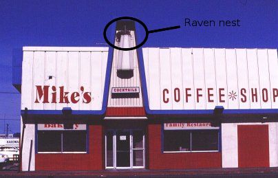
Second, ravens can choose to breed in a variety of different environments within the desert.
Towns in the desert give ravens access to artificial nest substrates (like the one on the left), as well
as food subsidies (like trash and road-killed carrion), as well as water sources. We'll call ravens
nesting in towns the "urban" population (granted, the town of Mojave, CA, is stretching the definition of
"urban").
Ravens nesting away from towns in undeveloped desert will typically nest in Joshua trees, which are the only
natural nest substrates in most places, or on cliffs if they are available. Away from towns ravens do not have
access to human food subsidies, and have to find naturally occurring foods. We'll call the ravens living in
undeveloped areas the "desert" population.
Between urban and desert habitats are undeveloped areas that are near enough to nest in natural substrates, but
be close enough to developments for ravens to have access to at least some human food and water resources. The
transition between two cover types is an "ecotone", so we will call these the "ecotonal" population.
Constructing a stage-structured population model for ravens in the Mojave
To construct a matrix model, we either need to be able to age the ravens, or at least be able to assign them to a
developmental stage. The stages that we use should be a) unambiguous, and b) internally homogeneous.
Ambiguous means unclear, or difficult to tell apart, so unambiguous stages are ones that we can tell apart for
sure. Ages have an unambiguous definition - a one year old is between its first and second birthday - but once a
raven is an adult, it isn't possible to tell its age anymore (a four year old and a ten year old look alike).
Since we don't know how old the ravens are, we can't use an age-structured model, so no Leslie matrix for us.
It is possible, however, to tell hatch year birds from juveniles, and juveniles from adults, so we can
use a stage-based model - we will use a Lefkovitch matrix to capture the stage structure in the
population.
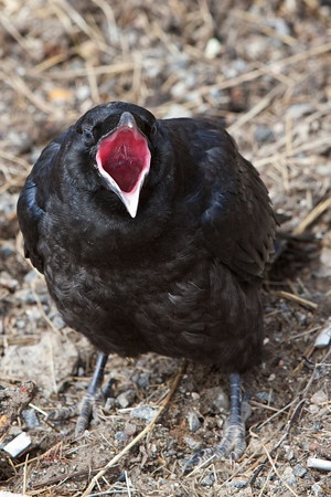
Hatch year ravens have pink mouth linings and gray irises.
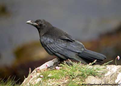
Juveniles have brown feathers in the wings and tail, instead of glossy black like adults have. The mouth
lining of juveniles is also pink, often through the second year of life. Juvenile eye color is in
transition from the gray color of hatch year birds to the brown color of adults over the first two years
of life as well. Between the plumage color and iris color it's possible to tell juveniles from adults
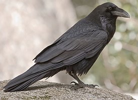
Adult ravens have glossy black feathers and brown irises. Once they become adults ravens can no longer be
reliably aged.
The stages we will recognize for this model will thus be the ones we can tell apart: hatch year, juvenile, and
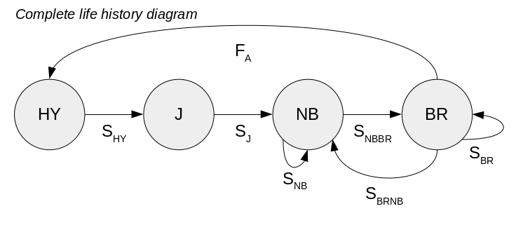
adult, with adults split between non-breeding and breeding. A diagram of this life history looks like the life
history diagram below.
The whole diagram is shown at first. Click once to see just the HY and J stages, connected by hatch
year survival (sHY). All of the juveniles come from HY birds that survive one year.
Click again and you'll see the transition from juvenile to non-breeding adult (NB). Juveniles that
survive one year become non-breeding adjult, with probability sJ. Non-breeding adults can
also survive more than one year, so there is a loop showing this - the proportion of NB adults who
survive and remain NB adults is sNB.
Click again, and you'll see that breeding adults (BR). Transition from NB to BR happens with a
probability of sNBBR. Breeding adults can also survive to breed again, with probability of sBR.
Some breeding adults survive, but lose their territories and become NB again, with a probability of sBRNB.
Finally, click once more and you'll see that breeding ravens produce all hatch-year ravens through
reproduction, at a fecundity per breeding female of FA.
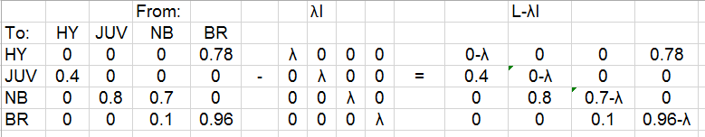
From this diagram, we can identify all the demographic rates needed for our Lekovitch matrix, and where they
should go.
From:
To:
HY
J
NB
BR
HY
0
0
0
FA
0.78
J
SHY
0.4
0
0
0
NB
0
SJ
0.8
SNB
0.7
SBRNB
0
BR
0
0
SNBBR
0.1
SBR
0.96
The first row of the matrix shows the contribution of each age class to HY birds. Since HY birds only
come from adults, the only entry will be to enter FA in the BR column. For the "urban" ravens
we'll be working with, this value is 0.78 female offspring per breeding female.
The second row shows the contribution of each age class to J birds. Juveniles come only from HY birds
that survive, so the only entry is sHY in the HY column.
The third row shows the contribution of each age class to NB birds. These non-breeding adults come
from juveniles that survive and become NB (sJ), NB adults that survive and remain as NB (sNB),
and BR adults that lose their territories and become NB (sBRNB).
The last row are the breeding adults - they come from non-breeding adults who gain a territory and
breed (sNBBR in the NB column), and breeding adults who survive and continue to be breeding
adults (sBR in the BR column).
All other entries are zero - for example, since NB adults don't breed there is no contribution of NB
to HY, so a 0 is entered in the NB column for the HY row. Although we have an entry for sBRNB
it too is set to 0 - that's because this is the matrix for urban ravens, which is the best breeding
habitat for the species in the desert, and breeding birds were not observed to lose their territories
and become non-breeders. This did happen in poor habitat, so we will have non-zero entries for sBRNB
in some of our Lefkovitch matrices, and the term is included here for completeness.
Note that some of these entries appear low because they are dividing a survival probabilities between two
different paths. For example, once ravens are in the non-breeding adult population their survival probability is
0.8, but this probability is split between the ravens that survive and remain non-breeders (0.7) and those that
survive and becoming breeders (0.1).
Population growth rate and stable age distribution of West Mojave ravens
If you download this file, you'll see that the first worksheet, Urban,
has this matrix in it.
Switch to the Ecotonal sheet and you'll see that ecotonal ravens have a lower hatch year survival and lower
fecundity than urban birds. Ecotonal adult survival probabilities are the same as in an urban population, but
breeding adults have a 10% chance of becoming non-breeders (thus, there is a SBRNB of 0.1, and a SBR of 0.86 for
the ecotonal ravens). Because the habitat is not as good for breeding in ecotonal areas, we will allow breeding
ravens to become non-breeders 10% of the time, but without suffering a survival cost of living in the ecotonal
areas.
In the Desert sheet you'll see that ravens living in the desert, away from human-provided resources, have lower
values still for hatch year survival, fecundity, and survival of breeders. Desert breeding ravens have an overall
survival probability of 0.8, and have a 10% chance of becoming non-breeders.
We will estimate the growth rate and stable age distribution for the urban population first, so switch to the
Urban tab.
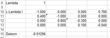
1. Set up the model for Solver. First, we need an initial value of λ - in cell A8 write
"Lambda", and in B8 enter a 1.
Next, we need to set up the formula for the characteristic equation of the matrix, det(L-λI) = 0,
which we will use to find λ. As you saw in lecture, L is the matrix of demographic rates, and λI is a matrix of
λ's on the main diagonal and 0's everywhere else, like this:
To keep our worksheet a little simpler, we can do the L-λI calculation in one step, without first making a λI
matrix, like so:
Enter the label "L-lambda I" in cell A10.
Enter =b3-$b$8 into B10. This will give you the 0-λ in the upper left corner of L-λI, and it will be equal to
-λ. Then, copy and paste this into the other diagonal elements - that is, in C11, D12, and E13. This should give
you -1 in C11 (which is 0-λ), -0.3 in D12 (0.4 - λ), and -0.04 in E13 (which is 0.96 - λ).
For the rest of the cells, we would be subtracting 0's in the off-diagonals of λI from the elements in the
off-diagonals of the demographic matrix, so we can just point to the elements in the demographic matrix. In cell
B11 enter =b4. Then copy and paste this cell to the rest of the cells in B10 through E13 that are not already
holding a value (that is, don't paste over the main diagonal you just created, but paste into the rest of the
cells).
Now we need to calculate the matrix determinant. We learned how to do these by hand in the lecture with a 2x2
matrix, but determinants are much more complicated for a 4x4 matrix - happily, there is a spreadsheet formula that
will calculate it for us. In cell B15 enter =mdeterm(b10:e13). Note that this is a matrix operation, but it works
on a single matrix and returns a single value, so it doesn't have to be an array formula. Label this with
"Determ." in cell A15.
Your layout should look like this:
2. Use Solver to find lambda. To find the growth rate you just need to start up Solver, and
have it set the determinant (in cell B15) to 0 by changing lambda (in cell B8). You should get a lambda of 1.0309,
which indicates a 3.1% increase per year in the urban population. You now have an estimate of population trend
that isn't based on any sort of abundance measure.
Be careful, though, because this could be an eigenvalue of the matrix but still not be the population growth
rate. There are actually as many eigenvalues as there are age classes, so it's possible to end up with Solver
finding one of these other eigenvalues instead. Since the growth rate is the largest positive eigenvalue, you can
double-check that you have it by setting lambda to 1.5 and running Solver again (a 50% increase per year would be
explosive population growth, which is not what we see - starting above any reasonable value and letting Solver
work down to it ensures that Solver's solution is the largest eigenvalue).
3. Calculate the stable age distribution. Now that we know the growth rate, we can estimate the
stable stage distribution. Each eigenvalue (such as λ) has an eigenvector that satisfies this
relationship:
Lw = λw
where w is the eigenvector (a column vector, meaning that it is a matrix with a single column). This equation is
telling us that the eigenvector, w, can be matrix multiplied by our demographic matrix, L, or can have each
element multiplied by our lambda estimate, and the results will be the same.
In cell G2 write "Stable stage". Enter starting values for the four stages of 0.4, 0.3, 0.2, 0.1 into cells G3
through G6 - we will have Solver change these, so the values don't matter too much, we just need a starting
point that isn't too far from the final values.
In cell i2 write "Lw". We're going to do a matrix multiplication of the demographic rates by the stable stage
distribution column vector. The result of a matrix multiplication is a matrix with the number of rows of the
left matrix (4), and the number of columns of the right matrix (1), and we need to select the entire output
range first, then type the mmult() formula, then do CTRL+SHIFT+ENTER to make it an array formula, like so:
Next we will multiply lambda by each cell in the stable stage column. In cell J2 enter "lambda w", and in J3
use the formula =b$8*g3. Copy and paste this to the rest of the rows, J4 through J6.
The Lw and Lambda w numbers will be the same once we find our stable stage distribution, but they are
different now because the values in G3-G6 aren't the right numbers yet. We now need a cell that compares them.
In cell i8 write "SS", and in cell i9 enter =sum((i3:i6-j3:j6)^2), and hit CTRL+SHIFT+ENTER to make it an array
formula. This formula subtracts the Lambda w column from the Lw column and squares the differences, then sums
them up. If you did this right the number is 0.16447. Once we have found our stable stage distribution this SS
cell will be 0.
We also want our stable stage distribution to be on a proportional scale, which means that the elements will
sum to 1. In cell G8 enter "Sum to 1", and in G9 enter =sum(g3:g6). We'll use this as a constraint in Solver.
Now to get the eigenvector with our stable age distribution. Start Solver, and use the following settings (see
the video for a walk-through):
Use the SS cell in i9 as the objective, and have Solver set its value to 0.
Use the stable stage numbers in G3 through G6 as the values to change.
Add a constraint - make Solver set the sum in G9 to equal 1.
Make sure the box is checked to make unconstrained variables non-negative (we want only positive values for
our stable stage distribution).
Run Solver, and the solution you get is the stable stage distribution.
You now have the population growth rate, and know the distribution of ages that is needed for change in
population size to be smooth over time.
4. Use the Urban setup to model ecotonal and desert areas. Now that you have the setup, you can
copy/paste all of the calculations to the other two sheets (don't paste special as values, you want the formulas -
just a plain copy and paste will do). Make sure you paste them in the same locations in Ecotonal and Desert as
they are in Urban so he cell references all point to the right places.
The other two populations are set up now, but since the demographic rates are different you need to run Solve to
get the correct lambda and stable age distribution for each.
Switch to Ecotonal and run Solver to set the determinant to 0 by changing lambda - this with a new set of
demographic rates we'll have a new growth rate.
To get the new stable age distribution, run Solver again, and set the SS cell to 0 by changing the Stable
stage values, subject to the constraint that Sum to 1 (G9) equals 1.
Then repeat these steps for Desert.
The population growth rates for the ecotonal and desert populations are both below 1, which means that these two
populations are declining. Or at least they would be, based on the balance of births and deaths represented in the
demographic matrices, but the regional population as a whole is propped up by the increasing growth rate of the
urban birds. Breeding territories are limited in supply, and once they are full the surplus ravens produced in
urban areas are not all able to find breeding territories there. The surplus produced by the urban population has
to disperse out into ecotonal and desert sites to find territories, and even though conditions are not as good
there, they at least have a chance to breed. This is a classic source-sink system, in which a large regional
population is being supported by surplus production within the source.
Optional for Biol 420, required for Biol 620 - using population models to evaluate management alternatives
The rest of the activity is about using these models to evaluate options for managing raven population size in
the desert.
Project the raven population over time
Considering the problems that unnaturally large population sizes of ravens cause for desert tortoises and other
sensitive species, we might want to explore some potential ways to reduce the productivity of the urban
population.
One way to evaluate the effects of various possible approaches to reducing growth rate in the urban population is
to use population projection. As a baseline for comparison, we can project the population using the actual
demographic rates and a starting population at stable age distribution. Then, we can see how population growth
changes when we alter demographic rates, or change the numbers of ravens in each age class for the starting
population. We really only need to do this for the urban birds, since urban areas are the source population for
the region.
1. Duplicate the Urban worksheet. First, let's make a copy of the Urban worksheet that we can
mess around with.
Right-click on the Urban tab, and select "Move or copy".
Select "(move to end)", and check the "Create a copy" box.
Rename the tab "Projection".
Switch to the Projection sheet, and delete everything except the matrix of demographic rates in A1 through E6.
In cell G2 enter "Pop. vector", and enter the numbers 27, 11, 26, and 36 - these are the stable age distribution
values multiplied by 100 and rounded to a whole number, so our starting population is as close to stable age as we
can get, aside from rounding error.
In cell H2 enter "t+1". You can then use the fill handle to extend to the right, which should increase the +1
part of the label - stop when you reach t+20 (column AA).
2. Project one year. This is a matrix multiplication of the demographic matrix by the
population vector, so we need a 4 x 1 output range selected - select cells H3:H6, and without changing the
selection type:
=mmult($b3:$e6, g3:g6)
and hit CTRL+SHIFT+ENTER to make this an array formula. The population vector for t+1 should now be in H3 through
H6.
You'll see that even though we have a growth rate over 1 we still had a slight decline in numbers for juveniles -
this is due to rounding error in the initial population sizes, nothing to worry about, things will settle down in
another couple of years.
3. Project to year 20. Using dollar signs to identify the matrix of demographic rates makes the
matrix multiplication copy and paste-able. Copy the cells in H3 to H6, and paste to i3, then continue to paste one
column at a time until you get to Year 20 in column AA. You have now projected the population twenty years.
You can calculate the total population size in row 8 - label F8 "Total N", and then in G8 sum the population
vector (G3 through G6). Copy and paste to the rest of the columns - these are the population sizes projected
through year 20.
Confirm that lambda is predicting growth rate - in cell F9 enter "Growth rate". In cell G9 enter =h8/g8, which
divides the population size at t+1 by the initial population size. Since Nt+1/Nt is what we
are trying to estimate with λ, we expect the number in G9 to equal our λ for urban of 1.0309. Copy this cell to
the rest of the projected years (H9 to Z9). Since rounding error prevented us from starting at exactly stable age
distribution the first calculation will be a little different from 1.0309, but after a couple of years the growth
rate will be 1.0309 and will stay at that number for the rest of the years. Because of this, it's possible to get
a growth rate estimate by projecting a population until it reaches stable age distribution, and then using the
ratio of population sizes to calculate λ.
4. Plot the numbers of individuals in each age class over time. Select cells G3 through AA6,
and plot a scatter plot with connecting lines. Time will be on the x-axis and population size is on the y-axis.
You should have a line for each age.
We should label the age classes - right-click and select data, and then switch row/column to get the series into
the horizontal axis box. Then click the "Edit" button under horizontal axis labels and select the names of the age
classes in cells A3 to A6. Once they are labeled, you can switch row/column again and the names will be retained
as the series names.
Add axis labels, and use "Year" for the x-axis, and "Number" for the y-axis. Add a title and call it "Population
projection".
Copy this graph by right-clicking and selecting "Copy". Then, paste a copy as a picture - right-click in a cell
of the worksheet and select the right-most icon of a clipboard with a picture on it. This makes a copy of the
graph that is no longer linked to the numbers in B3 through AA6, and will thus not change as you work through the
rest of the activity. This will be your baseline for comparison.
Evaluating management alternatives - changing numbers of ravens in each stage
We are projecting the population by multiplying a set of demographic rates by a population vector. To evaluate
various strategies for reducing growth rates for urban ravens, we just need to identify which demographic rate or
population vector number we would be affecting, and then change it.
For example, if we went out one year and knocked all of the nests we could find out of the trees, what would
happen to the raven population? Since the ravens could build nests again in the next year, and survival isn't
being affected at all, we wouldn't expect the demographic rates to change. Instead, this would be like reducing
the number of hatch year ravens to 0 in the first year.
1. Project the effect of removing a year of hatch year ravens. Change the number of hatch year
ravens to 0 for the first year - that is, change G3 to 0. You'll see in the graph that this causes a temporary
reduction in juveniles, since there are no hatch year ravens in the first year to replace the juvenile
mortalities, but this effect evens out quickly. Also, the growth rates in row 9 change for a few years while the
population is re-establishing stable age distribution, but they never drop below 1.
Change the title to "No HY in year 0". Then right-click and copy the graph, then select cell A10 and right-click
and paste-special as a picture (MAKE SURE you use the picture option, or this graph will change as soon as you
make any other changes to the population).
2. Remove the breeding population for one year. Now we'll see what happens when we take out the
breeders - set the hatch year birds back to 27 (enter 27 in G3), and set the breeders to 0. This simulates a
one-time removal of the entire breeding population. You'll see the graph changes a lot - since we still only allow
10% of the non-breeding adults to enter the breeding population per year there is a slow replenishment of the
breeding population. With no breeders the hatch year birds drop to zero in the second year (t+1), and with no
hatch year birds the juveniles drop to 0 in the third year (t+2). This depletes the non-breeding population for
several years as well, starting in year 4 (t+3). Growth rate even drops well below 1 for the first couple of years
while there are too few hatch year birds produced to replace mortalities.
Even so, the distribution of age classes starts to recover and all of the stages are increasing in number again
by year 10.
Change the title on the graph to "No BR in year 0", and copy and paste-special as a picture below your first
graph.
There are a couple of important points to note about this part of the exercise:
Even a population with lambda over 1 can decline for a period of time if the population is not at stable age
distribution.
Even severely perturbed populations (i.e. ones in which all of the breeders are removed) can recover if the
demographic rates are not reduced.
This is actually to be expected - we calculated lambda from the matrix of demographic rates, without any
reference to the number of individuals in the population or in each age class, so growth rate is only dependent on
the demographic matrix. If we want to make the population decline, we would need to change the demographic rates.
Changing the demographic rates
Survival and reproductive rates are partially properties of the species and partially properties of the
environment they live in, so to reduce survival or reproduction you would need to make lasting changes to one or
the other of those characteristics. You could reduce reproduction by giving the birds birth control drugs, by
knocking nests out of trees every year, or by preventing nesting in artificial structures. You could change
survival probabilities by reducing the amount of food subsidies they get from us (e.g. preventing road kill or
cleaning it up rapidly, covering trash, getting homeowners to stop feeding their pets outside), or possibly by
using lethal animal control methods. To have a lasting effect on the demographic rates, these changes would have
to be applied consistently year after year, or they would be like a temporary reduction in the population vector
that quickly recovers.
Set the number of breeders back to 36. Now we will see if discouraging some of the breeders from breeding each
year is enough to cause the population to decline.
Imagine that we did various things to prevent nesting on artificial structures, like putting up these
bird spikes on ledges. We probably can't keep every raven from nesting anywhere in town, but perhaps we
could prevent 10% of the breeding population from nesting each year. Would that be enough to cause the
population to decline?
In cell E5 enter =0.1*0.96 - this will move 10% of the breeders into the non-breeding population each year, which
simulates the effect or our bird spikes. Then, in cell E6 enter =0.9*0.96 - this places the remaining 90% of the
surviving breeders back into the breeding population. You'll see that with a new set of rates the starting
population is no longer at stable age distribution, so there is not a smooth change initially, but after about
year 7 the age distribution stabilizes and the population begins to decline.
Change the title on the graph to "10% of BR become NB", and copy/paste special as a picture below the other two.
Bear in mind, our population project is a mathematical model of what would happen, and it isn't perfect. For
example, if we project this population far enough it would eventually die out completely, which should make you a
little skeptical. If 90% of the breeding population was still able to breed, why would the population go extinct?
In fact, what would probably happen instead is that the population would decline, but when it got small enough
that most breeding adults could find territories the rate of breeders moving into the non-breeder category would
decline to zero again, and the population would stabilize at a smaller size. If we really wanted to cause a
decline that persists over time we would need to take away additional breeding sites every year, so that 10% of
the potential breeders would continue to be forced into the non-breeding population even as the population
declined, until there were no more breeding sites left. Our matrix model doesn't have any way to account for these
sorts of density-dependent changes, so a projection of the population assumes that all of the demographic rates
stay the same as the population increases or decreases.
That's it! Save your worksheet for your report.
By the way, there are programs (like Matlab and R) that can do the eigenanalysis we need with a few commands. We
will use Excel today, in part because you already know how to use it, and in part because it's easier to see what
the analysis is actually doing if you work through it in Excel. If you're interested, once you're done with the
analysis in Excel you can see the commands needed to do the analysis in R here.