Lab 2 - image interpretation, and digitizing features

In the first lab we worked with pre-existing vector data. The layers we used showed the land uses within the San Dieguito River watershed in either 1990 or 2016, but we used them without really thinking about where they came from. Today we will start to learn about how layers like that would be created.

The basic process is simple in principle, but complex and difficult in practice. Conceptually, the process is simply to identify patches of land with a single cover type, and then draw a polygon around it. Child's play, right?

There are actually several different ways you could create a vector cover type map:

• You could use GPS to record your position as you walked around the perimeter of each cover type patch in the field.
• You could use a statistical method of classifying cover type from images (air photos, satellite images), and then convert the image-based pixels to polygons.
• You could use air photos or satellite images on a computer screen, identify land cover types on them, and then draw around them on the computer.

We won't use the GPS method in this class - obviously, that would be a very time consuming and laborious way of mapping something the size of the San Dieguito River watershed, and is only really practical for smaller areas. Generally, if this sort of approach is used it's to fix mistakes made with one of the other two methods. We will learn how to do the second method in a couple of weeks - it is the fastest way to cover type a large area, but is prone to mistakes and requires extensive error checking and correction after the fact.

Today we will focus on the third approach, in which we will interpret the cover types from aerial images, and then draw (or digitize) the boundaries around them by hand. This approach is less prone to errors than the statistical classification method, but it involves a greater amount of subjective judgment - you will need to decide what the cover type you're looking at is, and where its boundaries lie. Digitizing by hand can be a very accurate and repeatable method if it's done by experienced people. We will just do enough today to learn the basics, but it can take a lot of training and practice to become proficient.

Some issues in digitizing features

Bear in mind that when we make a map we are producing an abstract representation of reality. There will be ways in which the representation will be wrong, no matter how we do the mapping. The trick is to do the mapping in a way that captures the features of the landscape that matter to the map's users, with as little distortion as possible.

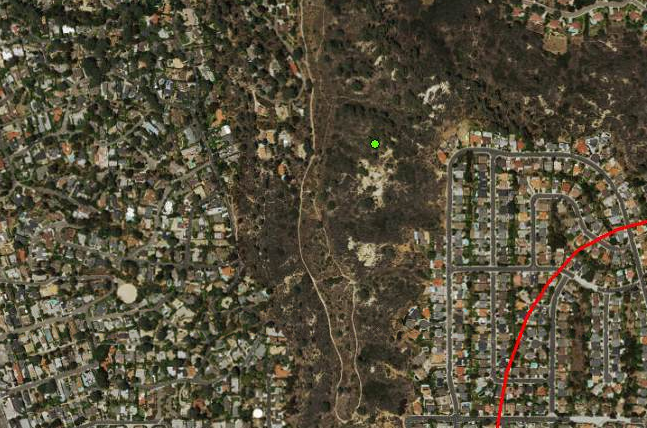
Let's start by looking at a high-resolution image of the Crest Canyon reserve, near the mouth of the San Dieguito River watershed.

You can see from this image that this is a complex area, with a mix of cover types we could map. There are a couple of housing developments on either side of the canyon, and the canyon itself runs from bottom to top in the middle of the image. The way that we would create a cover type map from this image would be to draw polygons that enclose contiguous patches of the same cover type. To draw a polygon you need to draw the edges, but where exactly are they? For the edges between housing development and undeveloped land we should be able to follow the property lines - there are fences there that are pretty obvious in the image. But what about within the canyon? Most of the canyon is vegetated, but you'll see that there is a green dot in the image next to a bare area - should we consider that a distinct feature, and draw a polygon around it? Or should we just decide the bare area is too small to consider a separate feature, and just draw a polygon around the entire undeveloped canyon? Alternatively, if we choose to map it, where exactly does bare patch end and vegetation begin?

This raises a couple of distinct problems:

• We need a classification system - that is, we need to decide what our cover types will be. Is all developed land the same thing? Or do we make a distinction between commercial development and housing areas? Between older housing developments with mature trees, and new developments with less mature landscaping? As for undeveloped land, do we make a distinction between woodland (sparse trees with shrubs or grasses between), shrubland, and bare ground, or is all of it just one "undeveloped land" category?
• We need to select a minimum mapping unit - that is, we need to decide how big a feature needs to be for us to map it. The smallest feature we will map is our MMU.

The classification system issue is something that is usually driven by the expected uses of the map. If all we were interested in doing with our map is to monitor development of land over time within the San Dieguito River watershed between 1990 and 2016, we would only need two categories: developed and undeveloped. We would then digitize these two types of land cover for each of these two years, and compare them - any land that was undeveloped in the 1990 map but was developed in the 2016 map must have been developed during that time period. Using so few categories may be too coarse, though - it might be good to know what kind of vegetation had been present, and what kind of development was going on in the region. We would then need to have different categories of undeveloped land (such as different vegetation types), as well as different categories of development (commercial, agricultural, residential).

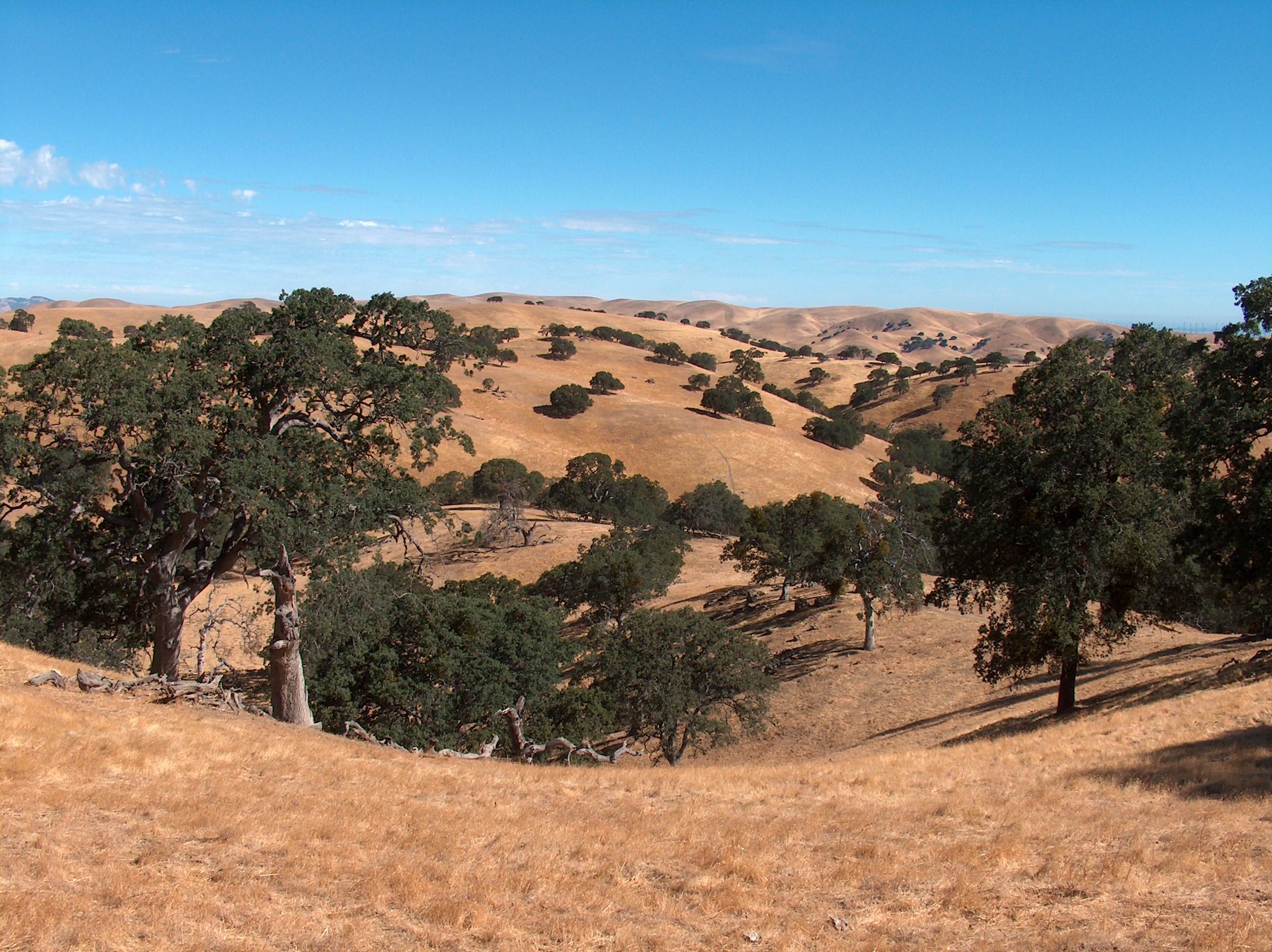
Once we know what the categories will be, we need to operationally define them. For example,consider this picture showing live oaks growing among fields of grass. This type of vegetation is called a woodland, which is defined as trees growing at a low density, with grasses growing in the spaces between them. We might consider everything in this picture to be one patch of oak woodland, but there are areas with high enough densities of trees that the tree crowns touch, and other areas where single trees are growing alone. We would need to define oak woodland relative to the lowest density allowed (below which we get grassland with an occasional tree thrown in) and the highest density allowed (above which we get forest). Depending on how we define a woodland, this entire area may be part of one woodland polygon, or there may be a mix of grassland, woodland, and forest polygons instead. Regardless of the choice, each category we use would need to be defined in an objective, repeatable way so that anyone mapping the area could map it the same way that we would have. In general, if different mappers interpret categories differently, and come up with different maps for the same area, that's a bad thing.

Bear in mind that the more fine-grained your categories are, the more work you have to do. Any time you have a transition from one cover type to another you need to draw the boundary between them. With more cover types there will be more boundaries to draw. On the other hand, it's possible to take a detailed map with a fine-grained, detailed set of categories and lump them into coarser units, but you can't make a fine grained, detailed map out of one with only coarse categories in it because the fine-grained information is just not there. Because of this, mappers generally try to use the most fine-grained system that time and money will allow.

The MMU question is a matter of deciding the spatial resolution of the map. The term "spatial resolution" refers to the level of spatial detail that will be represented. Returning to the example of a our canyon in Del Mar, even if we are inclined to map bare patches as separate cover types, you can see lots of tiny little bare patches throughout the canyon, which we probably don't want to map. The bare patch near the green dot is about 0.68 hectares, so if we chose an MMU of 0.5 hectares we would need to map it, but all the tiny little bare patches that are just a few square meters would be below 0.5 ha, and you wouldn't need to map them. If our MMU was 1 hectare, that 0.68 ha bare patch would be too small to map, and we would just draw one polygon around the entire canyon. Like the choice of classification system, the choice of MMU depends on how the map is to be used - if you are mapping habitat for a species that needs bare patches between between 0.3 and 0.5 ha in size as foraging areas, you would need to map bare patches down to 0.3 ha in order to represent the habitat for that species.

Map cover type polygons at each point

For your lab activity today, you will draw polygons around patches of land cover at points that I selected for you, based on ESRI's World Imagery layer. The categories you should use are:

• Forest - dominated by trees, closed canopy (i.e. adjacent tree crowns touching, with little or no bare ground visible between them).
• Woodland - roughly even mix of grassland and tree, with trees spaced such that their crowns do not touch.
• Shrubland - dominated by shrubs.
• Grassland - dominated by grasses, with little or no woody vegetation.
• Housing development - residential development.
• Commercial development - any development dominated by structures, but that is not residential.
• Agriculture - farms, orchards, or ranches.

You shouldn't have any trouble identifying housing developments, commercial developments, and agriculture. Let's look at how to tell forests, woodlands, shrublands, and grasslands apart in an aerial image. This may seem simple, but it isn't always - viewed from above, you can't tell how tall a plant is, or whether it has a trunk, so you need to use other characteristics to figure out if you're looking at trees or shrubs.

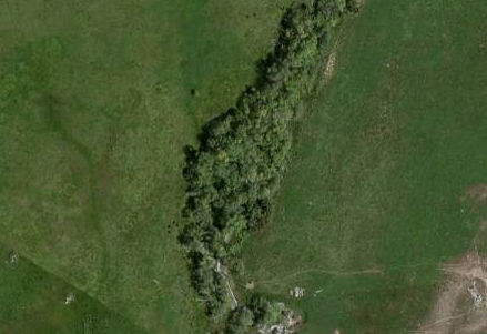
Here we have an image taken along a stream. The vegetation along streams is called "riparian vegetation", and it is generally dominated by deciduous trees in our region. There is clearly a difference between the riparian strip down the middle and the grasses around it, but the difference isn't color - both are about the same shade of green. The difference is in the texture. Because the trees are bigger plants than the grasses, you can make out individual trees in the image - individual trees have some spacing between them, and they cast shadows that are clearly visible, which gives the trees a coarser texture on the image. The  grassland looks more like a green carpet - there is some color variation, but individual blades of grass aren't discernible, and they blend together, which gives grassland a smoother appearance in the image.
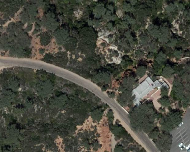
Here is a image of a portion of the Torrey Pines State Natural Reserve, showing a mix of trees and shrubs. Again, both the trees and shrubs are greenish gray, so color isn't much help in telling them apart. You can see from the size of the road and the building that the bigger plants have canopies that are 8-10 feet across or more, whereas the smaller plants are much smaller, perhaps 2-3 feet. The bigger plants are the Torrey pines, and the smaller ones are shrubs. Because shrubs are smaller and shorter than trees, they have a texture that's in between grasslands and forests.
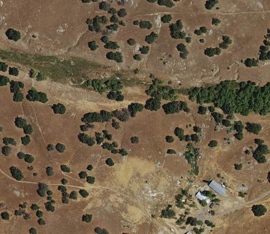
This is an example of oak woodland - the individual woody plants are big compared with the buildings in the image, indicating they're trees, they are growing sparsely, and they're surrounded by grasslands. Most of our grasslands are annuals, so they die back after the growing season and turn brown, so the color contrast will change depending on the season the image was obtained.

Okay, with that brief introduction to identifying cover types in mind, time to start digitizing.

1. Add a blank polygon layer to monitoring.mdb in ArcCatalog.

Start ArcCatalog and navigate to monitoring.mdb on your S: drive. The folder connections you created in Lab 1 should still be there, but if the folder connection to S: isn't present then recreate it (the instructions are in Lab 1 if you forgot how).

• Right-click on it and select "New" → "Feature class".
• In the window that pops up, give the layer the Name "cover_polys". You can leave "Alias" blank, and leave the "Type" set to "Polygon Features". Leave the Geometry Properties in their default, un-checked states. Click "Next".
• We will use the same coordinate system as the land use layers we worked with last time, so click on the "Add coordinate system button", , and select "Import". Navigate into your monitoring.mdb database and select landscape_open_space_1990 (which is the layer you imported last time), and click "Add". You should now see the Lambert Conformal Conic projection selected, with its coordinate system displayed below, which is what we want - click "Next".
• Accept the default tolerance - this has to do with how close together features have to be before their boundaries are automatically snapped together into one line. The default does a good job of keeping the lines where we want them, without leaving too many "sliver" polygons that are actually supposed to be the same line.
• The last step is to define the columns in the attribute table - you have two already (OBJECTID, and SHAPE), so now add a third with a field name of "cover", and a data type of "text". As you digitize the polygons you will enter their cover type in this column. Databases require us to specify the maximum size of an entry, which by default is 50 characters (including blanks) - as long as our categories are shorter than this 50 characters is fine (if we entered more than 50 characters the excess characters would be lost).
• Click "Finish", and you're ready to move on. If you get a warning about a "Geographic Coordinate Systems Warning", this has to do with the fact that the imagery layer and our cover type maps have a difference in their coordinate systems that needs to be accounted for - it's a minor problem that we can safely ignore here, so you can just click "Close".

2. Open ArcMap, and load layers

Start ArcMap, and create a new map (don't open the lab1 map).

Click on the "Add Data" button, and find the folder on P: with lab2 data in it. From the lab2 folder add Features_to_digitize.shp, ws_oneshape.shp, and "World_Imagery.lyr". The last layer is actually a file that points to some high-resolution imagery covering the entire surface of the planet, maintained by ESRI (the company that makes ArcGIS software). It displays as "Imagery" in your table of contents.

One odd feature of this World Imagery layer is that it's not a single data set, but rather it's several different images that are used at different magnifications. As you are trying to identify features you may find that zooming in and out doesn't just change the magnification, it causes an entirely different image to appear, taken in a different season and possibly in a different year. Sometimes you can make use of this to help you identify features - zooming in or out can give you additional information by giving you a look at the landscape in a different year or season.

Click the "Add Data" button again, and add the blank "cover_polys" layer you just created in monitoring.mdb.

3. Make the watershed fill transparent.

The watershed is going to define the boundary of our map, but it's also in the way of seeing the imagery. We can fix that.

• Double-click on the "ws_oneshape" layer in the table of contents, which will bring up the settings for the ws_oneshape layer.
• Switch to the "Symbology" tab - you'll see that it's set to use a single symbol, with a solid color fill. Click on the color in the "Symbol" area, and the "Symbol Selection" box will open.
• Within the symbol selection box, click on "Hollow" - it's the white square in the second row.
• You can pick an outline color that will stand out better too - drop down the "Outline Color" box and pick a nice bright yellow. Increase the outline width to 1 to make it show up better. Click "OK"
• Click "OK" to set the new symbol properties and return to the map.

You should now see the yellow outline of the watershed, but with no fill in the middle.

If you can't see the "Features_to_digitize" points on the map against the image, you can double-click on that layer and set the symbol size and fill color to something you can see (give it a try, it's pretty self-explanatory).

4. Zoom to the first point in Features_to_digitize.

Right-click on Features_to_digitize and open the attribute table. Click on the gray border on the left side of the first point to select it; you'll see it highlighted on the map. Then use the zoom in tool to zoom to the selected point (drag a box around it).

Now that you can see what land cover the point is in, identify the cover type as being one of the seven categories listed above, and look at where the edges of the polygon will be - you can consider roads and the watershed boundary to be edges, as well as any edge between the patch the point is in and any other cover type from the list.

The next step will be easier if you can see the entire patch of vegetation you will be drawing a polygon around - zoom in and out until you can see it all on your screen (remember, roads and other cover types are polygon edges).

5. Digitize the polygon.

First you need to turn on editing - select cover_polys, right-click, and select "Edit features" → "Start editing". If you get an error about ws_oneshape having different spatial references that's okay - the amount of error this causes in this map is small, and we are only using ws_oneshape as a boundary for the map, so if it's off a little it won't hurt anything.

You will see that an editing toolbar opens, like this:

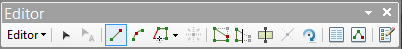
The last button in this toolbar is the "Create Features" button, and if you click it a new panel opens up to the right of your ArcMap window, titled "Create Features".

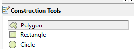
Select cover_polys, in the "Create Features" panel, and a set of "Construction Tools" should appear below. Select "Polygon":

To you use this tool you just need to click a point (called a vertex), then move your mouse (not drag, move) and you'll see a line between where you clicked and where your mouse pointer is located - click again and the next point is recorded, and moving the mouse starts to create a triangle. As you click along the edge of the patch of vegetation the polygon takes shape. When you're done you double-click, which completes the polygon.

A polygon is a set of vertexes that are connected by line segments, that enclose an area. To make the edge of the polygon follow the edge of the patch of vegetation accurately you need to put lots of vertexes along curved edges, but fewer are needed along straighter edges.

6. Enter the cover type in the attribute table.

Open the cover_polys attribute table, and enter the cover type you identified in the "cover" column.

You can close the attribute table between sessions of digitizing polygons, so close it now.

7. Repeat for the rest of the points.

Repeat this set of steps for each of the remaining points.

When you're done with all seven polygon, select the drop-down menu in the Editor toolbar, and select "Stop editing", and when prompted save your edits.

We are only going to do seven polygons, but that should be enough to give you an idea of the complexities of doing this kind of work. Imagine how long it would take to digitize the entire watershed, or the entire county!

When you are done, save a lab2 map file (with "File" → "Save").