So far we have emphasized using images for visually interpreting features. Even our false-color composites were
created to make it easy for a person to recognize different types of land cover in the image, but any
interpretation of cover types still required subjective judgment by a human observer about what they were seeing
on the screen.
Now we are going to begin using LandSat images to generate ecologically relevant data, without the need for subjective judgment by an analyst. Specifically, we will use LandSat to calculate the Normalized Difference Vegetation Index, or NDVI.
As you learned in lecture, NDVI takes advantage of differences in reflectance of visible red and near infrared EM radiation between healthy, actively photosynthesizing vegetation and unhealthy, dormant vegetation. NDVI is thus sometimes referred to as a greenness index. Calling NDVI a measure of greenness may seem odd, given that green visible light is not used at all in the calculation, but remember that green visible light isn't a reliable indicator of photosynthetic activity - a bright green football field that is covered with artificial turf is not "green" in the sense of being photosynthetically active.
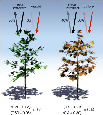
An example of how NDVI measures greenness of vegetation is shown in the illustration to the left - healthy, actively photosynthesizing vegetation reflects near infrared EM radiation strongly, but absorbs visible red light. In contrast, unhealthy, dormant vegetation still reflects near infrared radiation fairly strongly, but reflects much more visible red.
NDVI is a very simple calculation - for LandSat 5 images, that records red visible light with Band 3, and near infrared radiation with Band 4, NDVI is just:
NDVI = (Band 4 - Band 3) / (Band 4 + Band 3)
You can see example calculations in the illustration to the left, comparing a healthy green tree with a dormant tree. The difference in reflectance between Band 4 and Band 3 is a better indication of photosynthetic activity than either band by itself would be - the numerator of the NDVI calculation is thus the difference in reflectance between band 4 and band 3, and the difference will be bigger for actively photosynthesizing plants than for unhealthy or dormant plants of the same species.
But, the raw difference between the bands isn't sufficient for detecting differences in photosynthetic activity, because different species of plants reflect different overall amounts of near infrared or visible red EM radiation - this should not be surprising, given that different plant species may generally all be green, but the shade of green in their foliage is different. But, in addition to the obvious color differences between plant species, our Landsat pixels are recording more than just reflectance from a single species of plant. Each Landsat pixel covers a 30x30 m area, which will often contain a mix of different plant species, and may contain vegetated and unvegetated cover within the same pixel. Mixes of cover types affects the total amount of near IR and visible red radiation that is reflected in the first place, and the amount of difference possible between band 4 and band 3 is limited by the total reflectance for these bands (that is, the closer they are to 0 the smaller the difference can be). To adjust for differences in overall amount of reflectance the difference between near IR and visible red is divided by the sum of the near IR and visible red - dividing by a value to adjust for differences in total amount is referred to as normalizing the data, thus we are calculating a normalized difference. This normalized difference is used as a relative measure of greenness of vegetation, and thus we have a normalized difference vegetation index.
Today we will start by calculating NDVI the correct way, using reflectance. This will allow us to use the NDVI values to identify the general cover type (i.e. values less than 0.1 are usually barren, values between 0.2 and 0.3 are usually shrub and grassland, and values between 0.6 and 0.8 are usually wet, dense forests). We will do the needed calculations for the Spring of 2011, and will identify where in the watershed the NDVI was over 0.2 as a measure of vegetated cover.
ArcMap's Image Analysis tools include an easy to use NDVI button, but it is meant for display - the values that are created are NDVI values scaled to fall between 0 ad 255 so that they can be used as a color channel. We can't use these values to separate vegetated from unvegetated cover like we will with the reflectance-based NDVI calculations, but we can use them to visualize differences in NDVI between seasons, or within the same season across multiple years. We can use the Image Analysis NDVI button to give us a visualization of NDVI in the spring and fall of the same year, assign these to color channels in a composite image, and use color variation to illustrate seasonal change in greenness of vegetation. And, if we use the Image Analysis NDVI button to produce a layer for the spring of three different years we can composite them to visualize changes in greenness over time.
Note: starting today, the results of the analysis you do will be needed for your first mini project write-up.
Make sure you save the data sets you are told to save, as well as a map file for the day's activity, for later
use! If you lose work from today, you will need to do it again to complete the mini project assignment.
1. Load Band 3 and Band 4 for the Spring of 2011.
Start ArcMap with a new map, using monitoring.mdb as your default database.
We'll start by calculating NDVI the right way, using reflectance values instead of digital numbers (DN's). We only need band 3 and band 4 to calculate NDVI, so we'll only load those two bands.
Click on the "load data" button and selecting bands 3 and 4 for spring 2011 - they are on the P: drive, in the lab4 folder, then in folder sp11.
2. Calculate radiance for each band.
If you look at the bands in the table of contents, the color ramp used is grayscale, from black to white, with a low pixel value of 13 and a high value of 245 for Band 3, and a low of 7 and a high of 215 for Band 4. These values are digital numbers (DN), which are integer numbers between 0 and 255 that indicate the relative amount of light to emit from the computer screen when displaying the image.
To calculate NDVI, we will convert the digital numbers to radiance, which is the amount of light that was recorded by the sensors, and then convert radiance to reflectance, which is a unitless ratio of the proportion of light that struck the pixel that was reflected. We'll do this in two steps, starting with conversion of DN to radiance - this is a simple, linear formula:
radiance = (gain * DN) + bias
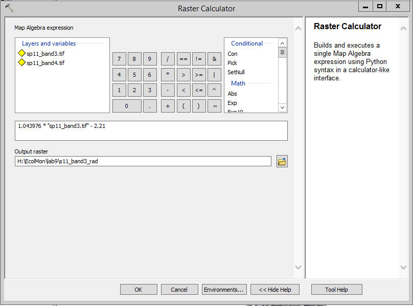
The band3 and band4 layers hold the DN's, so we will substitute the name of the band for DN when we do the calculation. There is a different gain and bias value for each layer, but they are constants, so once we know their values we can plug them in as single numbers. Gain and bias are properties of the sensors, and are updated periodically as the sensors aged - for example, the Band 3 gain in 2011 was 1.043976 and bias was -2.21 (All of the constants that we're using today come from this document, for your reference). Think of these numbers as adjustments that calibrate the sensors so that they produce consistent measurements over time.
We can do calculations like this with the raster calculator, which is part of the Spatial Analyst extension. Spatial Analyst is an optional add-on to ArcGIS that has most of the useful raster processing functions (remember, images are a type of raster GIS data).
Spatial Analyst is installed, but it may not be loaded by default - if you try to run any of the Spatial Analyst functions without loading it first you'll get an error message about a missing license file (not the actual problem, and thus a confusing and unhelpful error message). So, the first thing you should do is to make sure Spatial Analyst is loaded:
You should only have to do this once (but check that Spatial Analyst is turned on if you get weird error messages).
Now that it's activated, you can access the Spatial Analyst tools by clicking on the little red toolbox icon,  . You will get an "ArcToolbox" floating window, with lots of little
toolboxes. You can drag this window on top of the Table of Contents, and it will dock on top of it; you can then
switch between the Table of Contents and the ArcToolbox by selecting their tabs at the bottom of the window.
. You will get an "ArcToolbox" floating window, with lots of little
toolboxes. You can drag this window on top of the Table of Contents, and it will dock on top of it; you can then
switch between the Table of Contents and the ArcToolbox by selecting their tabs at the bottom of the window.
Find the Spatial Analyst Tools icon and click on the + to open it (not Spatial Statistics).
Now that you have the Spatial Analyst Tools open, find Map Algebra, and open it. Finally, double-click on "Raster Calculator". You will see a window like this:
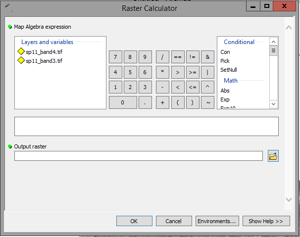
The Raster Calculator is used for doing calculations on raster layers (you may have guessed that from the name), such as the calculation of radiance from the DN's in our layers. Like with the query builder we used to select vector polygons based on their attributes, this tool is intended to help you build an expression by clicking on the numbers, operators, and names of raster layers you need to do a calculation - as you click along, your expression will be built in in the blank white field. You can in principle just type in formulas directly, but I'll warn you, ArcMap is fussy about formatting and not very good at reporting the causes of errors, and you will very likely make a typo that will cause your calculation to fail if you try to type the expression without using the graphical interface. At least for now, it's best to rely on the point and click approach.
We'll start with the calculation for Band 3 from spring of 2011.
Your final expression should look like (aside from using S: as the location of your output file):
It will take a few seconds, but as long as you see the progress notification at the bottom of the window:
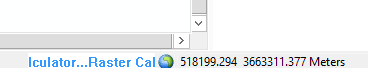
then you can assume it's still working, and wait for it to finish.
When the calculation is done you'll see a new s11_band3_rad image in your table of contents (you can switch to the table of contents tab to see the name). Notice that the legend showing the numbers associated with the shades of gray in the table of contents now goes from a low of 11.36 to a high of 253.56 - note that these are now decimal numbers instead of integer values.
You will need to repeat this calculation for band 4 for the Spring. The gain for Band 4 is 0.876024, and the bias is -2.39. Use s11_band4_rad as the output file name.
3. Calculate reflectance for each band.
Now that you have radiances for Band 3 and Band 4, you need to calculate reflectance. The formula is a little more complicated:
reflectance = (pi * radiance * d^2) / (E * sin(theta))
The terms on the right side are pi (3.14159), radiance (i.e. the results of our radiance calculation), d (the distance between the sun and the earth, in astronomical units (one astronomical unit is the average distance from the earth to the sun, so on average this value is 1, but varies slightly over time), E (band-specific radiance emitted by the sun), and theta (the solar elevation angle above the horizon at the time that the image was acquired). We know pi and radiance, and E is different for each band but has been constant for the period that data has been acquired. The values for E we will use are:
|
Band |
E |
|
Band 3 |
1536 |
|
Band 4 |
1031 |
The earth-sun distance need depends on the date - the "Julian" date is the number of days since the start of the year, so the combination of year and Julian date is used to find d, which is:
|
Date |
Julian date |
d |
|
4/15/2011 (spring 11) |
105 |
1.0033 |
The last piece that we need is theta, the solar elevation angle. This refers to how high the sun was in the sky
at the time the image was taken, and that will be different for every LandSat scene. The information is in a file
of metadata that's distributed with the images, which will have an MTL as the last three characters, and a .txt
extension. To look up the solar elevation angle from the MTL file, we need to start up ArcCatalog - click the
ArcCatalog button, 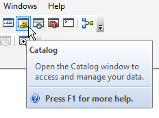 , to open it. Once it's open, navigate to
the lab4 folder on P:, and open the sp11 folder. You'll see that there are actually two files with MTL.txt as the
last characters, but one has an icon next to it that looks like a sheet of lined paper, and this is the one we
want to open - this is just a "text file" that has words and numbers in it. Double-click on the file to open it in
MS Notepad (Microsoft's text editor) so you can read it.
, to open it. Once it's open, navigate to
the lab4 folder on P:, and open the sp11 folder. You'll see that there are actually two files with MTL.txt as the
last characters, but one has an icon next to it that looks like a sheet of lined paper, and this is the one we
want to open - this is just a "text file" that has words and numbers in it. Double-click on the file to open it in
MS Notepad (Microsoft's text editor) so you can read it.
The formatting is a little messed up, but if you select "Format" → "Word wrap" you will see all of the information in the file. Select "Edit" → "Find" and search for SUN_ELEVATION. You'll see that the sun elevation when this image was acquired was 57.79040550 degrees above the horizon. You can close Notepad, as well as the ArcCatalog window.
Armed with these pieces of information, you're ready to calculate reflectance for each radiance band.
Start with radiance for band 3 in spring of 2011.
If all went well, your expression looks like this:
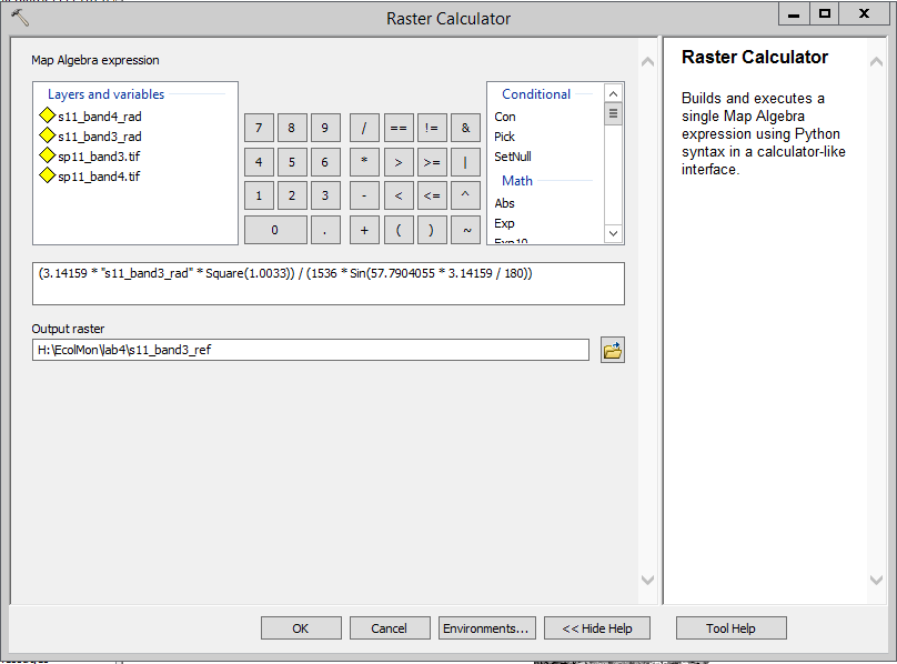
Click on "OK", and you in a few seconds you'll have a s11_band3_ref layer. If you did it correctly, you should have a low value of 0.027646 and a high of 0.616999 for your reflectance s11_band3_ref layer (if you don't get that double check your calculation - if they match out to several decimal places you're good to go).
**Note: if you need to re-do a calculation ArcMap will not let you overwrite an old file with a new file - you can open ArcCatalog and delete the layer created by the incorrect calculation first (find it in your output folder, right-click on it and delete it)**
You now will need to repeat this calculation for band 4. Considering that this was a complex formula that you don't want to have to type by hand again, it's a good idea to "recall" the calculation you just did and make the few modifications needed to apply it to Band 4. To do this you will need to find the "Results" window - it should open up as a tab along with the Table of Contents and ArcToolbox. Each ArcToolbox function you run adds an entry to the Results window, and the most recent one will be at the top (labeled "Raster calculator" [100..] or some similar number). If you double-click on this entry the Raster Calculator opens up again with all of the settings used for your s11_band3_ref calculation. To modify it to calculate reflectance to band 4 you just need to:
You don't need to change the distance or the sun angle, because both bands are from the same image, and pi and the conversion of angles to radians are the same. Click "OK" to get your Band 4 reflectances. The values should have a minimum of 0.013566, and a maximum of 0.67412.
Now you have reflectance for both of the bands, so you can calculate NDVI.
4. Calculate NDVI for spring of 2011.
We can now calculate NDVI. Open the raster calculator again and:
You'll see that the numbers you get for s11_ndvi are continuous, running from -0.39 to 0.85.
5. Change the color ramp so that high NDVI looks green.
By default, since NDVI is a single number, ArcMap uses a grayscale color ramp to display it. We can change this color scheme to something that makes it more obvious what the numbers mean.
Take a minute to look at the color variation - you'll see that water bodies have very low NDVI, and that there is variation in terrestrial areas during the spring. If you add the World_Imagery.lyr from Lab 2 to your map, and put the NDVI layer on top of it, you can use the Swipe tool from the Image Analysis window to see what kinds of cover tend to have low NDVI in the spring - you'll see that most are densely populated areas. Some of the highest NDVI values come from large irrigated lawns, like what you find in golf courses. Undeveloped shrublands have moderately high NDVI in the spring, since it is our rainy season.
6. Make a layer that shows vegetated areas.
Since we expect NDVI values over 0.2 to be vegetated, we can use the raster calculator to make a map that differentiates between vegetated and un-vegetated areas. To do this, start the Raster Calculator, and build the expression:
"sp11_ndvi" > 0.2
with the "Output raster" called "vegetated", inside of your monitoring.mdb database.
Using a comparison operator like =, < or > is a "logical test", and the Raster Calculator returns either "true" (which is a value of 1 to a computer), or "false" (which returns a value of 0). The resulting "vegetated" layer shows all the areas with NDVI over 0.2 in one color, and all the areas that are less than or equal to 0.2 in another.
7. Quantify the amount of vegetated area in the watershed.
If you right-click on the "vegetated" layer, you'll see you can open the attribute table. An attribute table for a raster data set is simple - it gives a row for each of the data values present in the raster map, and a count of the number of pixels that have that value. There are only two values in the "vegetated" layer, and you want to know how many are equal 1. Write that number down.
Next, to convert a number of cells into an area, you just need to multiply by the area of each cell. LandSat pixels are 30 m on a side, or 900 square meters. A hectare is 100 m on a side, or 10,000 square meters, so a 30 x 30 m pixel covers 900/10000 = 0.09 hectares. If you multiply the number of pixels with a 1 by 0.09 you will get the number of hectares of vegetated land in the watershed.
Note that although this method didn't require us to make any subjective judgments about the cover types we see, this is not a perfect method - golf courses and older housing areas with mature landscaping are being classified as "vegetated" using this method. We will learn another method of doing cover typing in our next class meeting that will do better at differentiating between undeveloped and developed land, but bear in mind that objective methods aren't always better when it comes to cover typing! Well trained mappers would not mistake housing developments for undeveloped vegetation.
We are now going to learn a quick and easy way to visualize seasonal change over time, by assigning NDVI layers to color channels on the monitor. The method of calculating NDVI you just learned is the best method to use for any sort of quantitative analysis, but we can't assign a "floating point" layer (i.e. one with decimal numbers) to a channel on the monitor, we need digital numbers for that.
To visualize change in NDVI over time we can Instead use the Image Analysis window's NDVI button to make layers that represent NDVI, but on a 0 - 255 scale that can be used for visualization.
Before you move on, you can right-click and remove from the table of contents all of the ref and rad layers, as well as the vegetated layer, and just leave your sp11_ndvi layer and the original .tif files. Removing layers from the TOC doesn't delete them from your S: drive, but it does get them out of the list of layers we have to choose from, which makes it easier to find the layers we want to use in the next steps.
1. Make an NDVI layer from the Image Analysis window for sp11 using the tif files.
Make sure the bands are in numeric order, with band3 above band4 in the table of contents.
In the Image Analysis window, select sp11_band3.tif and sp11_band4.tif, and then click on the NDVI button (the
maple leaf next to the composite button) 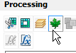 .
.
You'll see you have an NDVI layer with a color ramp assigned that makes high levels of NDVI green, and low levels orangeish brown. Doing it this way, the NDVI values are scaled to fall between 0 and 255, so we lose the numeric interpretation of the index, but it's still a useful way of seeing where the green areas are and where the barren areas are.
2. Make an NDVI layer for f11.
Do the same operation you did in the previous step for Fall 2011 - load the f11_band3.tif and f11_band4.tif layers, put them in numeric order, select them both in the Image Analysis window, and click on the NDVI button.
You should now have an NDVI_sp11_band3.tif and an NDVI_f11_band3.tif layer in your TOC. If you put them in order, with Spring 11 above Fall 11 and then use the swipe tool, you'll see that there is a big decrease in greenness in the fall in undeveloped areas - this makes sense since fall is our dry season.
3. Composite NDVI for spring and for fall.
Swiping is fine, but it's useful to be able to make a single image that shows the differences between two layers - we can do this by using the two NDVI layers in a composite, and then use color variation on the screen to tell us where the drying is happening between spring and fall.
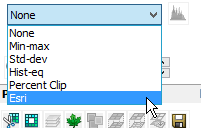 - click on the composite, drop down the histogram menu and select the "Esri"
method, which gives a good separation between the colors.
- click on the composite, drop down the histogram menu and select the "Esri"
method, which gives a good separation between the colors.You should now have a map with purple and green, as well as white, black, and shades of gray. To interpret what you're seeing, you need to think about how RGB color works:
We can extend this visualization approach to view changes in spring NDVI over time. We can calculate NDVI for the spring of 1984, the spring of 1998, and then composite those with the spring of 2011 to see how greenness has changed over this 27 year period.
1. Calculate NDVI for spring of 1984 and for 1998.
Add band 3 and band 4 for 1984 and for 1998 to the table of contents (they are in folders sp84 and sp98 in the lab4 folder of the P: drive). Put them in order so that band 3 is above band 4 for each year.
Select band 3 and 4 for spring of 1984 in the Image Analysis window, and make an NDVI layer. Repeat for spring of 1998.
2. Make an NDVI composite for 1984, 1998, and 2011.
Put the three spring NDVI layers in chronological order in the table of contents.
Select all three spring NDVI layers in the Image Analysis window, and make a composite. By default, this assigns 1984 to red, 1998 to green, and 2011 to blue.
Adjust the contrast if needed (use the Esri option in the histogram tool of the Image Analysis window).
To understand what you're looking at, remember how color works in the RGB model...the table below gives colors associated with several different combinations of R,G,B values, the pattern of land cover change that this represents, and the likely cause of the pattern of change.
|
Red (1984) |
Green (1998) |
Blue (2011) |
Color |
Land cover change indicated |
Likely cause? |
|
High |
High |
High |
No change - green in all three years |
Green vegetation all three years |
|
|
Low |
Low |
Low |
No change - not green in all three years |
Lack of vegetation all three years |
|
|
High |
High |
Low |
Vegetated areas became un-vegetated between 1998 and 2011 |
Loss of vegetation (due to development or fire) shortly before 2011 |
|
|
High |
Low |
Low |
Vegetated areas became un-vegetated between 1984 and 1998 |
Loss of vegetation due to development after 1984 (probably not fire, or vegetation would have recovered by 2011). |
|
|
Low |
Low |
High |
Un-vegetated areas grew vegetation between 1998 and 2011 |
New park, new agricultural field, new golf course - artificial, irrigated vegetation |
|
|
Low |
High |
Low |
Un-vegetated areas grew vegetation between 1984 and 2011, then became un-vegetated in 2011 |
Possibly due to fire before 1984, then again before 2011, with recovery in between. |
|
|
Low |
High |
High |
Un-vegetated areas grew vegetation between 1984 and 1998 |
Fire recovery after 1984, or new artificial vegetation |
|
|
High |
Low |
High |
Vegetated area became un-vegetated between 1984 and 1998, then became vegetated between 1998 and 2011 |
Fire just before 1998, or development followed by growth of new artificial vegetation |
See if you can find areas that have developed since 1984. To help you check, add the World Imagery layer we used in previous labs beneath the composite, and then use the swipe tool to see what the land cover looks like under the colors.
Don't forget to save a map file (lab4.mxd). Your monitoring.mdb database has your NDVI layer for the spring of 2011, and your map of vegetated areas according to spring NDVI, which you need for your report - this should all be in the database on your S: drive, and is thus saved already.
Also, bear in mind that your composites of seasonal change in NDVI, and of change over the time in NDVI are not permanently stored yet. If you want copies of these, you'll need to save them. For example:
You can save Composite_NDVI_sp84_band3.tif the same way - use a file name that indicates this is your composite
of spring NDVI for three years.