Analysis of field trip data - accuracy assessment
Today we will work on comparing data we collected in the field to the cover type maps we produced from LandSat
data (unsupervised classification map) or downloaded (landuse_2016_simple.shp).
There are a lot of steps needed to get this task done, but the task is conceptually simple. The basic road map
for the day is:
- Import GPS points into ArcMap
- Overlay the GPS points that indicate the actual cover type we observed in the field with the cover type maps
we have been working with
- Make a "confusion matrix" that compares what we observed in the field with what the maps say would be there.
There are multiple steps involved for each of these, which are given below.
Import GPS points into ArcMap
Calculating positions of points at a distance from the observer
The data from our field outing is in this file. Download it into your
S: drive.
If you open the file in Excel, you'll see that there are several columns:
- Point number - a unique, sequential ID number.
- Obs.East - the UTM East coordinate of our observation points recorded in the field from our GPS.
- Obs.North - the UTM North coordinate of our observation points recorded in the field from our GPS.
- Distance - the distance recorded with the range finders.
- Direction - the direction to the point recorded with the compasses.
- Description - the description of the feature recorded.
I did some checking, and a few points had data entry errors that placed them in wildly incorrect locations -
those have been dropped from the data set. We have 45 points that were accurate enough to use.
Before we can plot the points on the map, we need to calculate the locations from the GPS locations, distances,
and directions.
|
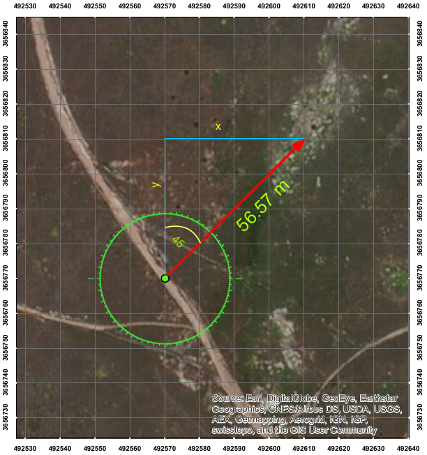
In the illustration to the left, we have a GPS location of 492570 E, 3656770 N, and from that point we
are recording the rock outcrop that is 56.57 m away, at 45°. We need to calculate the number (x) to add to
our known east coordinate, and the number (y) to add to our known north coordinate to get the coordinate
of the rock outcrop. You can see that the red line with our recorded distance forms a right triangle with
lines running due north and due east from the point (in blue), so we can use trigonometric functions to
figure out what we want to know.
Remember from your trigonometry class that the sin of an angle (A) is the opposite side of a right
triangle divided by the hypotenuse - the hypotenuse is the red line with our measured distance, which
we'll call D, so:
sin(A) = x/D
Solving for x we get:
x = D sin(A) = 56.57 sin(45) = 40.
Likewise, the cos of A is the adjacent side over the hypotenuse, so:
cos(A) = y/D
y = D cos(A) = 56.57 cos(45) = 40
|
Once we have these x and y values, we just add x to East and y to North to get our new coordinates - the new
coordinates are thus E + D sin (A), and N + D cos (A). You can see from the UTM grid that the rock pile is indeed
at 492610 E, 3656810 N, which is 40 m north and 40 m east of the original point.
To do these calculations on the data in Excel:
- Enter "East" into G1, and "North" into H1. These will be the UTM east and north coordinates for the feature we
are mapping.
- The first feature we are mapping is the rock outcrop in row 2. In cell G2, enter the formula
=b2+d2*sin(radians(e2)) - this is the east coordinate of the rock outcrop. Notice that this is just translating
the formulas for x and y above into Excel syntax, except for one thing - rather than just taking the sin of the
direction with sin(e2), we need to convert the direction from degrees to radians, which are the units that Excel
uses in all of its trig functions.
- You remember radians, right? Radians express angles in terms of the distance around a circle with a radius
of 1, which is 2π. An angle of 90 degrees is π/2 radians, an angle of 180 is π radians, and in general an
angle of A degrees is 2π * A / 360 radians, or (π * A / 180 radians, to simplify)).
- In cell H2, enter the formula =c2 + d2*cos(radians(e2)). This is the north coordinate of the rock outcrop.
- Copy and paste G2 and H2 to the rest of the rows.
Some points were recorded by standing at the feature and recording its location, and didn't require any
displacements to be added to them. We are dealing with this by using a 0 distance and direction for those points -
that way we can enter the calculation once, copy/paste for all the other rows, and get the correct result
regardless of whether the point is at a distance from the recorded GPS coordinate or not.
Converting field descriptions to cover types
When we overlay these points with cover type maps, we will only want to use the points that recorded a cover
type, and not the ones that recorded the un-mappable habitat features. We will use a column in Excel that we can
filter on later, so that we can just focus on the cover type points.
- In cell I1 type "Type", and then for each row enter either "Cover type" or "Feature". For example, rock
outcrops, fences, perch locations, and snags are all features. Shrub or scrub, bare ground, riparian, lake, and
developed are all cover types.
We will also want to use the same cover type categories as are in our land use vector maps, and in your
unsupervised classification cover type maps. There are two different systems that we used, so we'll need a column
for each:
- In cell J1 type "Cover", and then for every "Cover type" row record the cover type category used in your
unsupervised classification maps that matches the description. These are the nine cover types listed in the
instructions for Lab 5 (cover typing).
- In cell K1 type "LU", and then for every "Cover type" row record the land use category found in the
landuse_1990_simple.shp or landuse_2016_simple.shp files we used for change detection analysis last week. There
are 14 categories, but only a few pertain to the area we sampled - you can see what the land use categories are
in your transition matrices from last week.
As you do this, note that spelling counts - if you use different labels for the same thing it will make your work
harder later. Once you enter a cover type of land use category once, copy it and paste it wherever else you need
it to ensure that you enter things the same way every time.
Save the Excel file onto your S: drive, and quit Excel. MAKE SURE YOU QUIT EXCEL or ArcMap will refuse to open
the file.
Importing GPS data into ArcMap
Now, to import the GPS data from the Excel file into a point layer. Start up ArcMap with a blank map, and do the
following:
- You can add data from an Excel spreadsheet like you would a map layer - click on the "Add Data" button and go
find the spreadsheet, then double-click the file name to see a list of the worksheets within it. You'll see that
there is only one worksheet, called "FieldPts$" - select it and click "Add".
- We haven't told ArcMap which columns to use as spatial coordinates yet, so there's nothing plotted on the map,
but you should see "FieldPts$" in your table of contents (note that adding a data table that can't be mapped
switches the table of contents to "List by Source" mode, so the locations of all the files is given as well as
the file names).
- Right-click on the "FieldPts$" entry, and select "Display XY Data". In the "Display XY Data" field that pops
up:
- Set the "X Field" to"East"
- Set the "Y Field" to "North"
- Click "Edit..." to set the coordinate system - we need to tell ArcMap that these are UTM coordinates.
- Open "Projected Coordinate Systems" → "UTM" → "WGS 1984" → "Northern Hemisphere" → "WGS 1984 UTM Zone
11N".
- Click "OK" to set the coordinate system for the points.
- Click "OK" to display the coordinates. You will get a warning that the table does not have an Object ID
field, which is okay for now (we'll fix that in the next step), so click OK.
- You will now have a new layer in your table of contents called "FieldPts$Events", which is plotted on the map
as points. You can right-click on FieldPts$Events and zoom to it to see the points.
- We need to convert these to a layer in your Biol420.mdb database now so that we can do the overlays we want to
do. Right-click on FieldPts$Events, and select "Data" → "Export data". Set the "Output feature class" to go into
your Biol420.mdb file, with a name of "field_points", and click "OK".
If you switch to "List by Drawing Order" mode in the table of contents, you can drag the points above the imagery
layer. You can also label the points by their descriptions - double-click on "field_points", and switch to the
"Labels" tab. Check the box to "Label features in this layer", and set the "Text string" to "Label Field:" of
"Description". Set the color of the label test to a nice bright yellow, and click "OK". You'll new see the labels
for each point on the map.
You can right-click and remove "FieldPts$Events", and "FieldPts$", you don't need them now that you have a map
layer of that data.
Now that we have field points and their attributes, we need to overlay them with our cover type maps to see how
well the cover type maps reflect what we find on the ground.
Overlay GPS points with cover type maps
Add the landuse_2016_simple.shp file from the lab7 folder, and your unsupervised classification map that you
re-classified into our nine cover types (which should be called "cover_spring11" in your biol420.mdb file). You
can also add the "World Imagery.lyr" file as background.
Extract cover types from your unsupervised classification cover type map
Now we can extract cover type categories from the cover_spring11 map, using the field points to identify which
pixels to record - for each point, we will get a row in an output table that records the pixel value it touches.
- In the "Arc Toolbox", locate "Spatial Analyst Tools" → "Extraction" → "Sample", and launch the tool.
- Set your unsupervised cover type map as the "Input rasters", and "field_points" as the "Input location raster
or point features". The output table can go to your S: drive, as a table called "field_unsup" (with no extension
- this will make ArcMap use its own data table format, which does a better job of preserving the names of the
fields in the attribute table).
- Click "OK" to run the tool.
The Sample tool makes a table, but does not make a new point layer, so nothing new will be on the map. You will
see a table called "field_unsup" in your table of contents, though. If you open the field_unsup, you'll see there
is a column called "FIELD_POINTS" that gives the point number from the field_points layer, and a column called
"SP11_COVER" that gives the cover types. We need to add these columns back into the field_points file, which we
can do by "joining" the tables.
Joining database tables is done based on matching entries in each table. Once they are joined, the columns from
both tables can be displayed and used as though they were a single table. To join "field_unsup" to the attribute
table of "field_points", do the following:
- Right-click on "field_points", and select "Joins and relates" → "Join".
- In the "Join Data" window, set:
- "1. Choose the field in this layer that the join will be based on:" to "OBJECTID"
- "2. Choose the table to join to this layer, or load the table from disk:" to "field_unsup"
- "3. Choose the field in the table to base the join on" to "FIELD_POINTS"
- Click "OK" to join the tables.
If you right-click on field_points and open the attribute table, you'll see that there are now columns at the end
that come from field_unsup, including the one that gives the cover type code from SP11_COVER.
Extract land uses from landuse_2016_simple
Joins don't permanently join columns to an attribute table, they just link files for use temporarily. But, the
join does persist if we use the joined file in an operation that makes a new output file. We'll take advantage of
that now to overlay field_points (and its joined field_unsup table) with landuse_2016_simple to make a new point
layer with an attribute table that has the cover types we observed in the field (from field_points), the cover
types in the cover_sp11 map (from the joined field_unsup table), and from the land use map for 2016 (from
landuse_2016_simple). That attribute table will have everything we need to compare what we observed in the field
to either of the maps.
To do the overlay:
- Select "Geoprocessing" → "Intersect". An intersection is like the union operation we used in our change
detection exercise, except that only the overlapping features are retained - since we only want information
about the land use polygons that the points fall into, this is a better choice for our purposes.
- In the "Intersect" window:
- Select "field_points" and "landuse_2016_simple" as the "Input features".
- Set the output feature class to go to your biol420.mdb database, and call it "field_vs_maps"
- Click "OK" to run the intersection.
You will get a new point layer added, field_vs_maps, in your table of contents. If you right-click and open the
attribute table, you'll see that you now have the LU_current field appended to the end.
While you have the attribute table open, we can simplify the next step if we "turn off" columns that we don't
need for making our confusion matrices. For example, we don't need to know the feature ID numbers from various
files we used along the way - position your pointer over the column label "FID_field_points_field_unsup",
right-click, and select "Turn field off". This hides the field from view, and will also prevent it from being
exported. You can repeat this with every column except:
- Description
- Type_
- Cover
- LU
- field_unsup:SP11_COVER
- LU_current
If you make a mistake and turn off the wrong thing, you'll need to drop down the menu in the upper-left corner of
the Table window and select "Turn All Fields On" and start again.
We are going to convert the field_vs_maps file to an Excel spreadsheet so we can do our confusion matrix
calculations using PivotTables.
By the way, you may have noticed we worked a little differently today than in previous labs - so far we have only
used ArcGIS table file format or have generated point layers within our biol420.mdb database, but have not used
the dbf file format (either as an output table in Sample, or indirectly by creating a shapefile as an output layer
in our intersection operation - remember, shapefiles use dbf as the format for attribute tables). We needed to
avoid dbf files because our field names are long and descriptive, but the dbf format only allows 8 characters for
field names. If we used a dbf file as an output table, or used a shapefile as an output point layer format, our
field names would all have been changed to something that fits in 8 characters, no matter how unintelligible the
new name is. If we go straight form an ArcGIS table to an Excel file, all the field names will be preserved.
Now, to export the field_vs_maps attribute table directly to an Excel spreadsheet file, do the following:
- In the ArcToolbox, open "Conversion Tools" → "Excel", and then launch "Table to Excel".
- Select as the "Input Table" your "field_vs_maps" layer.
- Put the output Excel file on your S: drive, and call it "field_vs_maps" (an xls extension will be added
automatically).
- Click "OK" to run the conversion tool.
Make a "confusion matrix" that compares what we observed in the field to what the map says would be there
Open field_vs_maps.xls in Excel. You'll see that the only columns in the spreadsheet are the ones we left turned
on in the attribute table for field_vs_maps.
We are going to make a confusion matrix for each of the maps - we'll start with the unsupervised classification
map.
- Insert a PivotTable, and drag "field_unsup_SP11_COVER" into the ROWS. This is what the map says is at each
point, and you will see your numeric codes
- Drag "field_points_Cover" into the COLUMNS. This is what we actually saw in the field, translated into one of
our nine cover types.
- Drag "field_points_Cover" again into VALUES, and make sure the value field setting is "Count" (it should be by
default).
- Drag "field_points_TYPE_" into FILTERS
Make a new worksheet for your results - click on the plus in the circle to make a new worksheet. Re-name the
sheet to "Confusion". Switch back to your pivot table in Sheet1.
You can drop down the list in cell B1 and just show "Cover type" rows. Copy the cells in your pivot table
(starting with cell A4, and including enough cells to get the row and column totals), and paste-special as values
into cell A3 in your new worksheet. In cell A1 type "Confusion matrix - unsupervised classification". You can now
replace the row labels with the cover type names as you assigned them (you should have saved an Excel file that
gave the numbers you assigned, and the cover type names associated with them).
Now we'll do the land use categories from landuse_2016_simple.shp:
- Switch back to your pivot table on sheet 1, and click inside of it to bring up the layout window.
- Drag all the fields out of ROWS, COLUMNS, and VALUES.
- Put "LU_current" into the ROWS
- Put "field_points_LU" into "COLUMNS", and again into "VALUES".
You should now have a confusion matrix showing the mapped land uses in landuse_2016_simple.shp (rows) compared
with what we saw in the field (columns). Copy and paste-special to cell A20 of the Confusion sheet, and label cell
A18 "Confusion matrix - land use".
MAKE SURE YOUR ROW AND COLUMN LABELS ARE THE SAME ON YOUR CONFUSION MATRIX
It's possible that there might be some cover types on your map that we didn't see in the field, or cover types we
saw in the field that weren't mapped. The accuracy statistics instructions assume that you have the same set of
cover types in your rows and columns, and if that isn't true make it so before you move on.
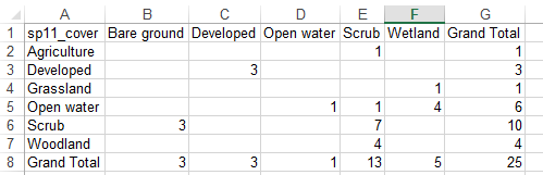
| So, for example, if you have something like this... |
|
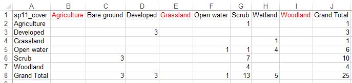
| ...add blank columns for cover types that are in the rows but not the columns... |
|
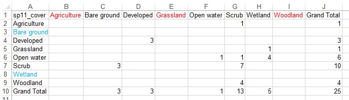
| ...and blank rows for cover types that are in the columns but not the rows. The labels should match when
you're done |
|
| As a last step before going on to the accuracy statistics, update the row and column totals. In this
example, to sum the Agriculture row, in cell B10 I would enter =sum(b2:b9), and to update the Agriculture
row I would enter =sum(a2:i2). These could then be copied and pasted to the rest of the rows and columns. |
Accuracy statistics
Now to calculate the accuracy statistics for the maps. For each of your confusion matrices, make sure the rows
and columns are sorted in the same order so that the matches are on the main diagonal. Then do the following:
- Overall accuracy - four cells below the bottom of your confusion matrix, type "Overall accuracy", and in the
cell next to it enter a formula that sums the matches, and then divides by the total number of points.
- Label the column two over from the end of your confusion matrix "Producer's accuracy", and then in each row
divide the matches by the row totals.
- Label the row two down from the bottom of your confusion matrix "User's accuracy", and then divide the matches
by the column totals.
Do this for each confusion matrix. It's possible that students will have different numbers of rows and columns,
depending on how they assigned the point descriptions to cover types, so I can't give you specific instructions
for which cells to use, or what the formulas will be. Try coming up with the formulas yourself, and I'll help if
you run into trouble.
Look over the mis-classifications for each map - look down the columns to see which cover types were hard to map
accurately, and to see what cover types were incorrectly assigned to each cover type. Look across the rows to see
what the mapped cover types proved to be when we checked in the field - what mistakes did each method make? And,
think about the mis-classifications in terms of two possible causes: 1) changes over time, such that the map was
accurate when it was made but it now no longer reflects conditions on the ground, and 2) mapping errors. It may
not always be obvious, but a point that was mapped as developed land and found in the field to be undeveloped is
probably a mapping error - it is very unlikely that houses were converted to undeveloped land. The opposite (land
that is mapped as undeveloped, but was found to be developed) is more likely to be an actual change on the ground
- we would have to find out when the development was done to be certain, but it's much more plausible from first
principles.
That's it! Save your confusion matrix spreadsheet, you'll be using it in your project write-ups.