Why use randomization testing?
In your statistics class you learned a variety of powerful methods for testing for differences between treatment groups (i.e. t-tests, analysis of variance), and for relationships between two continuous variables (i.e. regression, correlation). Although these techniques are the best available when you meet the assumptions they make about your data, they can give incorrect results if your data don't meet the assumptions.
There are several assumptions that must be met to use these techniques:
-
Independence of observations
-
Normality of data
-
Homogeneous variances (between groups, or of residuals)
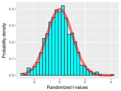
When we're doing statistical hypothesis testing, a probability distribution is used as a mathematical model of how random samples from a population should behave. The t-distribution is a good model for the distribution of means of samples taken from a population, or of differences between two random samples from the same distribution - it's therefore called a sampling distribution. If we meet the assumptions the t-distribution is based on, we can use it to calculate the probability of observing differences between our treatment and control group means by random chance - this probability is called the p-value. If we don't meet the assumptions of the t-test, then the t-distribution is no longer a good model for random sampling from a population, and if we use it as a sampling distribution to obtain a p-value, we will probably not get accurate results.
When you don't meet the assumptions of a particular test, though, all is not lost. It's possible to use a resampling approach to generate a sampling distribution just from the data in hand, without reference to any mathematical model of sampling from a population. The histogram shows 1,000 t-values generated by randomly shuffling the data between two groups from a single sample, and you can see that the distribution of t-values is roughly bell-shaped, to the point that the t-distribution superimposed on it in red matches fairly closely. We can thus use the set of 1,000 differences in place of a t-distribution to calculate p-values.
Resampling approaches are appropriate for a very wide array of analytical problems in Biology, and can be used in place of all the common techniques you've learned in your stat class. These techniques make no specific assumptions about the distribution of the data, don't require that the distributions are the same between groups, and don't even require that the data points are independent of one another. The only assumption they make is that the sample in hand provides the best information available about the distribution of data in the population as a whole. When your data meet the assumptions of a t-test, ANOVA, or regression, then randomization tests will be slightly less powerful (i.e. slightly less likely to detect a real experimental effect), so you are better off using the standard techniques. But, when your data don't meet these tests' assumptions, you are better off using a resampling approach.
We will use randomization tests today as an example of the resampling approach to hypothesis testing. Randomization testing is not a standard part of commonly used statistical software, but it's not too difficult to implement the technique using macros in Excel.
A randomization test for differences between two means
The data we will use was included as an example in Whitlock and Schluter's "The Analysis of Biological Data".
During mating, sockeye salmon males are bright red due to carotenoid pigments found in the food they eat. Salmon are not able to synthesize carotenoids themselves. Kokanee salmon are landlocked sockeye salmon that live their entire lives in fresh water; they spend their adulthood in a lake, then spawn in streams and rivers that feed the lake.
Carotenoid pigments are not as common in fresh water as they are in salt water foods, yet kokanee males are red during the breeding season just like sockeye males. Researchers interested in how kokanee manage to turn red when they have little access to carotenoids hypothesized that they may be more efficient at storing carotenoids than their ocean-run relatives. They established two different groups of fish in aquaria, ocean-run male sockeye and male kokanee. They fed both on the same diet with low levels of carotenoid pigments. After the males reached maturity they measured their color using a colorimeter (an electric device that measures the intensity and wavelength of colors). The colorimeter wavelengths are then represented as a "color score" which indicates the redness of the value; the larger the value the more brightly red is the male. Your task is to test whether kokanee are brighter red than male sockeye when fed a diet poor in carotenoids.
|
So, we need to use a randomization test instead, because we can't assume normality or HOV. To know whether our results are likely to be just due to random sampling, we need to know how different two samples can be just due to random chance. To know this, we need many, many random samples, but we only have one. How do we generate the random samples we need? |
|
|
|
|
|
So, it's starting to look like the difference we observed is pretty unlikely to occur by random chance. |
|
So, what we should expect is that over many random re-shuffles of data to species type, we will rarely if ever see differences between random groupings that are bigger than what we actually observed. If we count up the number of times we see bigger differences in random groups than in our actual groups, we can divide this by the number of random re-groupings we produced, and this will give us the probability of seeing a difference as big as we observed by random chance. |
The general procedure you will use to test for this difference will be:
- Measure the actual difference between groups using an appropriate test statistic, and record it
- Randomly sort the color data, but not the salmon species, so that color index values are randomly assigned to species
- Measure the difference in randomly assigned color scores between salmon species using the same test statistic, and record it
- Repeat many times (1,000)
- Count the number of times that randomly generated differences are as great or greater than the observed difference (plus 1), then divide by the number of randomly generated differences (plus 1) - this is your p-value
- If p < 0.05, reject the null hypothesis of no difference between sockeye and kokanee colors - look at the
means to determine which species is redder
We'll do a couple of variations on the same procedure to give you a chance to check your understanding of the program. For this first step, though, we'll set up the spreadsheet and do the initial recording of the macro. Next time we'll add the loop and set up recording of the results.
Step 1 - download this file, save it where you save files, and open it.
The file format is a "macro-enabled worksheet", and has the file extension "xlsm". Macros are very useful, but they can also be used to deliver computer viruses, so Microsoft has made a different version of its spreadsheet file format in which macros can be used. This gives users some warning that the sheet they are about to open has macros in it that can be run when opened - if the user isn't expecting a macro to be in the file, they can choose not to open it to avoid infecting their computers. If macros are stored in the standard file format, they can be opened and viewed, but they won't run.
You'll see that there are two columns, one identifying the species (kokanee or sockeye), and the other giving the skin color measurement.
Step 2 - generate the summary statistics needed for the test.
Use a pivot table to calculate three summary statistics for each species: mean skin color score, standard
deviation of skin color score, and sample size. Use species as row labels, and have each summary statistic in a
different column. Put the pivot table in the Two Group sheet, starting in cell A40. When you're done, it should
look like this .
.
It's possible to turn off the annoying "GetPivotData" function that crops up when you select a cell from a pivot table. Select the File menu in the upper left corner of the sheet, then select "Options" from the bottom of the menu. Switch to the "Formulas" tab, and un-check the "Use GetPivotData functions for PivotTable references" option in "Working with formulas". You will now be able to click on cells within a pivot table and just get the cell reference returned.
Step 3 - calculate the observed test statistic.
Even though we can't use the t-distribution to calculate our p-value, we can still use the t test statistic as a convenient measure of how different the groups are. The t-statistic measures how many standard errors are between the group means.
In cell E40 type "Pooled variance". In cell E41 calculate the pooled variance for both kokanee and sockeye. This is the variance of the difference between the means. The formula for pooled variance is:

Translate this into a spreadsheet formula - n1 and s1 are kokanee standard deviation and sample sizes, n1 and s1 are sockeye standard deviations and sample sizes, and n1 + n2 is the total sample size. If all goes well you'll get a value of 0.044087.
Next, type "Pooled standard error" into cell F40, and in F41 calculate the pooled standard error. The formula is:

This will equal 0.071244 if entered correctly.
Finally, in cell G40 type "t", and in G41 calculate the observed t-value. The formula is:

..which will be equal to 10.31891. Since you have not yet randomly shuffled the data, this is the actual observed t-value. Copy it and paste-special the cell value to cell A47, then type "Observed t" in cell A46.
Step 4 - set up the data for random shuffling.
Randomization tests are done by randomly shuffling the data - that is, the same set of skin color values are used every time, but the are randomly re-assigned to either the kokanee or sockeye groups by randomly sorting the data values while leaving the species labels in place. Each data value is only used once, and the sample sizes stay the same for each group for each shuffle.
- Enter an original order column - in cell C1 type "Original order", then in the cells below number from 1 to 35. You can do this quickly by typing a 1 in cell C2, selecting cells C2 to C36, then selecting "Fill" → "Series..." from the right side of the "Home" tab. The default option is a "linear" series with a step value of 1, meaning that it will increase by 1 for every selected row.
- Type "Randomizer" in cell D1
- In cell D2 type in the "rand()" function, which will give you a random uniform number between 0 and 1 with 15 decimal places of precision. Copy and paste the rand function to cells d2 through d36.
You will use the randomizer column to sort the skin color and original order columns, but not the species column. Because this is a function it will re-calculate each time the worksheet changes, so we can randomly shuffle the data repeatedly by sorting on this column again and again. You will probably not see the random numbers in order, because the sorting and re-calculating happens so quickly that a new set of random numbers appears before you can see the old set sorted in order.
Step 5 - set up a column to record the randomized t-values.
In cell I1 type "Randomized t-values". It's important to use column I, because as the test runs we will be filling in 1000 rows for this column, and we don't want to write over part of the pivot table, or the t-value calculation, which are in columns E through G.
Step 6 - record the macro.
You are now ready to use Excel's macro recorder to record the procedure you will use for each repetition. You might want to run through the instructions in the bulleted list below without the macro recorder on so that you know what you're going to do - the recorder will record everything you do, including if you select the wrong cells or scroll around trying to figure out where things are, and all these actions will leave some unneeded steps in your macro that will slow down its execution later.
Once you're sure you know what you need to do, click on "Macros" from the "View" tab and then "Record macro". Call the macro "RandTest", and assign it the shortcut key of capital R (ctrl+shift+R). Use the default "Store macro in this workbook" option. You can write in a description as well - something like "Randomization test for color differences between kokanee and sockeye salmon".
Now, while the macro recorder is on, do the following:
-
Select cells B1 through D36 - this omits the species names, but that's intentional...it's very important that you NOT select the species. Switch to the Home tab, and under "Sort and Filter" select "Custom sort". Sort the data on the "Randomizer" column. This will randomly sort the color index values and the original order values, while leaving the species unsorted.
-
Click into the pivot table, then right-click and select "Refresh". This will update the pivot table with a new set of averages and standard deviations, and will also cause the t-value to recalculate.
-
Select the t-value in cell G41, right-click, and copy.
-
Select cell I2, right-click and paste-special "Values".
-
In the "View" tab, click on "Macros" and turn off the macro recorder.
If all goes well, you now have the set of steps needed in each iteration to generate a new random re-grouping of the data, and to record the t-value that results. Next time we will modify the macro to repeat this operation a bunch of times.
Assignment
That's it for now - save the file and we'll work with it next time to conduct the analyses.
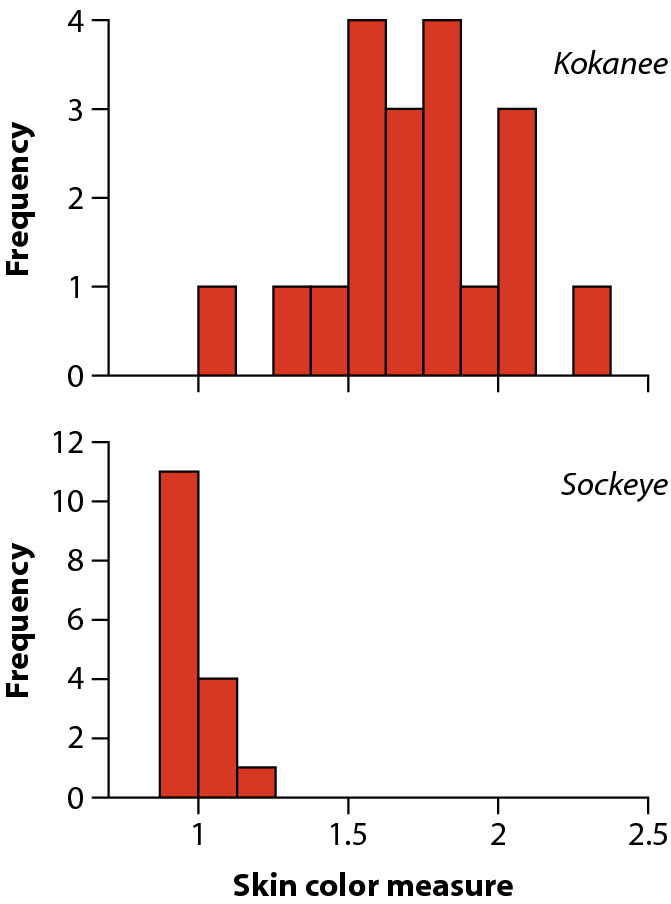 The histograms to the left should give you an idea of why a t-test is not a good choice -
the color measurements have very different distributions between the two species, with very different
variances, and the sockeye distribution is nowhere near normal. If we were to test for lack of normality
(with an Anderson-Darling test) and lack of HOV (with a Levene's test) we would fail both tests.
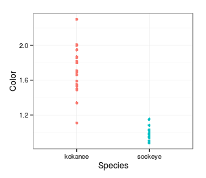 The way that randomization
tests get around this problem is very clever. First, we start by realizing that if there really isn't
any difference in skin color between kokanee and sockeye males, then calling them "kokanee" and
"sockeye" is arbitrary - it's a distinction without a difference. If that's right, then essentially the
names are randomly assigned to the skin color numbers, and randomly re-assigning them should give us
differences in means that are essentially the same as what we actually see. For example, here is a graph
showing the actual distribution of skin color measurements for the two groups. The mean for kokanee is
1.72, and for sockeye it's 0.99, for a difference of 0.73. It looks like sockeyes tend to be less red,
but this could be due to random chance. What would the data look like if we randomly assigned data
values to salmon species?
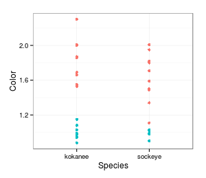 Here's one such random
assignments. The color of the points still indicates the actual species, but the position along the
x-axis indicates the group the data points are assigned to - you can see some kokanee are assigned to
the sockeye group and vice versa. The mean for the random grouping is 1.39 for kokanee and 1.39 for
sockeye, for a difference of 0. This is a much smaller difference than before, so it makes the actual
amount of difference we observed look big compared to random chance. But, we can't tell much from just
one random shuffle, so let's shuffle again.
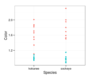 This random shuffle also makes the
observed data look pretty non-random - the mean for kokanee is 1.39, and the mean for sockeye is 1.38,
for a difference of 0.01.
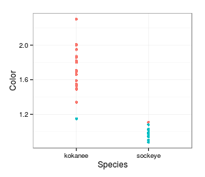 But, lest we jump to conclusions,
here is a possible grouping of the data that would give an even bigger difference than we saw in our
observed data - you see that there was one sockeye male that was redder than on kokanee male, and when
we switch those two data points we get means of 1.72 and 0.98, for a difference of 0.94 - just slightly
more than actually observed.