We will be working today with an approach to statistical inference based on comparisons of models that each represent scientific hypotheses, rather than on null hypothesis tests. The goal of this kind of analysis is to find which hypothesis is best supported by the data. This approach is called the method of support, or MOS for short.
Our approach throughout all but the last couple of weeks of the semester has been to test a single null hypothesis. With a null hypothesis test we assume the null is true, calculate the probability of obtaining our results if the null is true, and if the probability is low we reject the null in favor of an unspecified alternative hypothesis. This procedure seems to set up a competition between two different hypotheses, the null and the alternative, but these two hypotheses are conceptually very different. The null hypothesis says that there is exactly 0 difference between group means (or that the slope of a regression line is exactly 0), whereas the alternative hypothesis is just that the null is incorrect. When we reject the null a difference of exactly 0 is evidently not well supported by the data, but we have not done anything to evaluate the support for any other amount of difference specifically - treating evidence against one hypothesis as though it's evidence for another is a logical fallacy called a false dichotomy.
The MOS is very different. With the MOS it isn't possible to test a single hypothesis alone, like we do with a null hypothesis, because we can't draw any conclusions at all from a single model. Instead, we need to compare models to one another to draw any conclusions.
There are several important points to bear in mind about the MOS:
-
It is model based, which means that we have to be able to express our hypotheses as models. For example, we learned in our classic model selection exercise that:
-
If a predictor variable is included in the model, we are hypothesizing that the response depends on it. Conversely, if a predictor is excluded, we are hypothesizing that the response is independent of it.
-
If we lump two or more levels of a categorical grouping variable together into one, we are hypothesizing that the two different levels have the same mean. If we split a single level into two or more different levels, we are hypothesizing that each new level has a different mean.
-
If we include a quadratic, cubic, or other higher-order term for a predictor, we are hypothesizing that the response has this specific non-linear relationship with the predictor.
-
If we include an interaction between two predictors we are hypothesizing that the response to one predictor depends on the level of the other.
-
-
Support for hypotheses is assessed at the level of the model. To assess the importance of a specific variable, or a model term (such as an interaction) you must fit models that include the variable/term and others that do not, and assess which model is best supported by the data.
-
Model-based inference only works if the same response data are used for every model. Any set of predictors can be included, and models can be compared even if they contain completely different sets of predictors. Specific cases that would be problematic are:
-
A missing value from one of the predictor variables causes R to drop the entire row of data from the analysis, including the response variable's data value. If some models use the entire data set and others are missing a data point or two, you shouldn't compare the models.
-
The response variable needs to be on the same scale for all of the models - you can use an untransformed response variable for every model, or a transformed response variable for every model, but they all must be the same. You can, however, transform only some of your predictors, and can even compare a model with a transformed predictor to one with the un-transformed version of the same predictor as two separate hypotheses.
-
-
We have to assume a distribution of residuals around the model to calculate likelihoods and AIC values, so we should assess the usual GLM assumptions for any model we wish to interpret. Models that are poorly supported that don't meet GLM assumptions are not a problem, but any model that is well enough supported that we wish to interpret it should meet GLM assumptions.
- The end result of this approach is not a "test" of a hypothesis in the sense that there is no binary pass/fail decision made about the hypothesis. Measures of support for hypotheses, such as AIC's and model weights, are meant as relative measures, which we should use to gauge the strength of our confidence in our conclusions.
-
Measures of support do not substitute for measures of model fit or effect size, such as R2, because the best-supported model in the set we are considering could still be lousy. We should also always include an intercept only model to check the "no effect" hypothesis - only models that are better supported than the "no effect" model should be considered for interpretation.
Although this method can be used to analyze any data set, it is most attractive for studies in which the null hypothesis is not plausible. As we discussed in lecture, this covers nearly all ecological studies, and any lab study in which random allocation of subjects to treatments is not possible, such as differences due to species, sexes, ages, genotypes, and so on.
Today's exercise - the brain/body size relationship
This exercise will be based on brain weight and body weight for a variety of species of animals. Most are mammals, but there are three dinosaurs included (their data come from estimated values, based on the sizes of their skeletons).
Start a new R Studio project in a new folder. The data set we will use today is here, and the Rmd file is here. Import the data into a dataset called "brains".
If you look at the way the data are organized you will see that it contains data on the log of brain mass, the log of body mass, the identity of the species (Species column), and four different hypothetical groupings of the species:
- dinosaurs separate from mammals, mammals grouped by Order (column Taxa)
- dinosaurs separated from non-dinosaurs (column Dino.nodino)
- primates separated from non-primates (column Primate.noprimate)
- dinosaurs and primates get their own groups, and all other mammal species are lumped together (column Dino.prim.other)
Work through the instructions in the tabs below to answer the questions about confidence intervals for a proportion in your Rmd file.
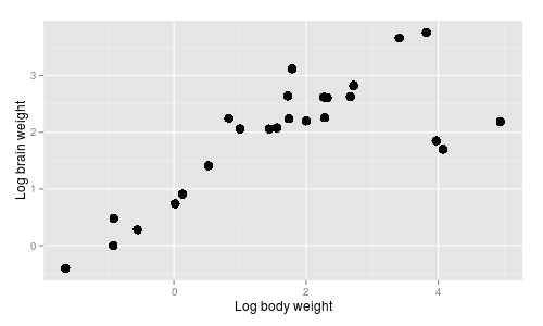 The brain/body data is shown in the graph to the right. Brain and body weight have both been log-transformed,
which makes the relationship linear...which, by the way, tells you that brain and body weight have what kind of relationship? Click here
to see if you're right
The brain/body data is shown in the graph to the right. Brain and body weight have both been log-transformed,
which makes the relationship linear...which, by the way, tells you that brain and body weight have what kind of relationship? Click here
to see if you're right
You can see that there is a general, positive relationship between body size and brain size, which makes sense - a large part of the mass of the brain is devoted to simply operating the body, and large bodies require large brains to operate them.
For this exercise, we are interested in finding a model that best represents the brain size/body size relationships of these species. To give you an idea of how this will work, let's look at a couple of examples of hypotheses we could evaluate.
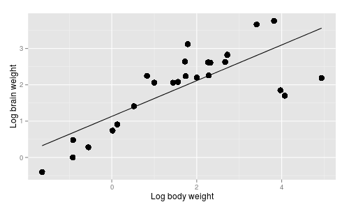 One possibility is that brain/body scaling is the same for all species, regardless of the taxonomic group they
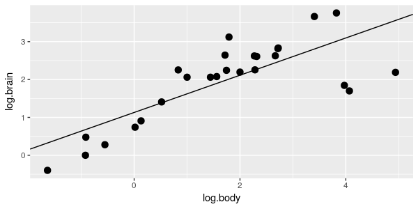
belong to, and a simple linear regression of log.brain on log.body would represent this hypothesis, like the graph to the right.
One possibility is that brain/body scaling is the same for all species, regardless of the taxonomic group they
belong to, and a simple linear regression of log.brain on log.body would represent this hypothesis, like the graph to the right.
The AICc value for this model is -16.89.
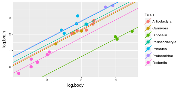
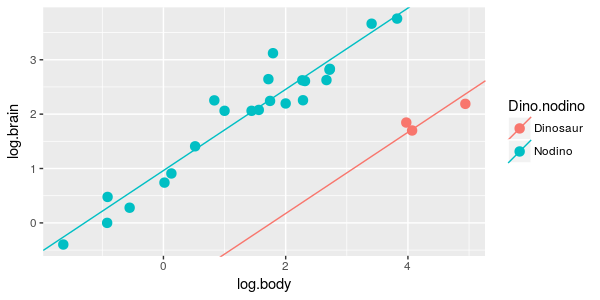 The cluster of three data points that are separate from the rest of the data are the dinosaurs. Dinosaurs are
notoriously small brained, but it's possible that the change in brain weight per unit change in body weight is the same for mammals and dinosaurs. If that's true, then a single, common
slope may apply to both the dinosaurs and the mammals, and each taxa only needs a different intercept to represent the overall differences in brain size. You probably recognize this
version of a linear model as an ANCOVA.
The cluster of three data points that are separate from the rest of the data are the dinosaurs. Dinosaurs are
notoriously small brained, but it's possible that the change in brain weight per unit change in body weight is the same for mammals and dinosaurs. If that's true, then a single, common
slope may apply to both the dinosaurs and the mammals, and each taxa only needs a different intercept to represent the overall differences in brain size. You probably recognize this
version of a linear model as an ANCOVA.
It certainly looks like a separate line is desirable for the dinosaurs, and not surprisingly the AICc for this model of -57.21 is substantially lower than for the single line hypothesis above. This model is the better of the two we have looked at so far, and if we subtract the AICc for this model from each of the first two, we would get a ΔAICc of 0 for this model, and 40.31 for the single line model. With just these first two models to consider, the simple linear regression can be safely disregarded in favor of this ANCOVA model.
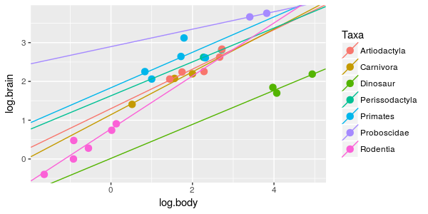
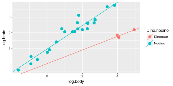 Alternatively, it could be that the dinosaurs not only have different brain sizes on average, they may also have a
different rate of change in brain tissue with increasing body size. If this is the case we need an interaction between log.body and Dino.nodino to allow each group to have a line with a
different slope and intercept. This model is illustrated to the right.
Alternatively, it could be that the dinosaurs not only have different brain sizes on average, they may also have a
different rate of change in brain tissue with increasing body size. If this is the case we need an interaction between log.body and Dino.nodino to allow each group to have a line with a
different slope and intercept. This model is illustrated to the right.
This model also looks pretty good, but we had to add an additional parameter to produce the differences in slope. The AICc value for this model is -56.98, not quite as small as the previous one. The previous model with parallel lines is still best supported (with a ΔAICc of 0), and this model with different slopes has a ΔAICc is 2.13.
With just these three models to go on we could confidently conclude that dinosaurs and mammals are different enough to need their own lines (ΔAICc is huge for the model with a single line), but whether their scaling relationships have the same slope or different slopes is less certain (ΔAICc = 2.13 for the model that includes an interaction between log body weight and dino.nodino).
We will implement these three models, and six more that use the other grouping variables in the data set to determine which hypotheses are well supported by the data, and which are poorly supported.
Instructions:
1. Fit all the models. We will fit several models to compare with one another, and need to collect them all in a list, just like we did when we were using adjusted R2 to analyze caloric content of foods. To start, we will create an empty list into which we can add our fitted models. Use the command (in the make.models.list of your Rmd file):
models.list <- list()
Now each time we fit a model we will add it as a named element of our models.list object.
For example, the hypothesis that there is a single brain/body scaling relationship for all of these species is a simple linear regression of log.brain on log.body (in the log.brain.on.log.body chunk of your Rmd file):
models.list$body.lm <- lm(log.brain~log.body, data = brains)
By assigning the output of the lm() statement to models.list$body.lm we create a named element called body.lm within the models.list object, and store the fitted model within it.
That takes care of the first hypothesis' model, out of a total of 10 hypotheses we will compare. Since the MOS uses models to represent hypotheses, the translation of scientific hypothesis first to a type of linear model, and then to an R model formula to use in the lm() function, is shown for each hypothesis in the table below. It is structured like so:
- The scientific hypothesis is stated first, expressed in scientific terms, in the "Scientific hypothesis" column
- The hypothesis is then translated into the type of linear model that would be used to represent the hypothetical relationship between variables stated in the Scientific hypothesis column. If you hover over the "Hypothesis as a linear model" for a hypothesis a graph pops up to show what the lm will look like
- The model formula you will use in R to represent the model is shown next, in the "R model formula" column. The model formula to use is displayed for the first two models (the first one being the body.lm model you already assigned to models.list). For the third to tenth model the model formula is hidden until you click "What is the model?" - take a moment to construct the model formula yourself before looking at the answer, it will give you useful practice for when you have to do this on your own
- The name of the model to use when you assign the lm to models.list is given last, in the "Name of model to use" column. The model name aren't critical, but the rest of the instructions will be easier to follow if you stick with these names
Go ahead and fit the 2nd through 10th models, adding each to your models.list (in the fit.remaining.models chunk of the Rmd file).
| Scientific hypothesis | Hypothesis as a linear model (hover for graph) | R model formula: | Name of model to use |
|---|---|---|---|
| 1. There is a single common brain/body scaling relationship for all species in the set. |
Simple linear regression of log.brain on log.body
 |
log.brain ~ log.body |
body.lm |
| 2. The scaling of brain size and body size is the same for all species, but taxa differ in their average brain sizes for their body size. |
ANCOVA of log.brain by taxa, with log.body as a covariate
 |
log.brain ~ log.body + Taxa |
taxa.lm |
| 3. Each taxa has a different scaling relationship. |
ANCOVA of log.brain on taxa and log.body, with an interaction between log.body and taxa.
 |
What is the model? | taxa.int.lm |
| 4. Brain/body scaling is the same for dinosaurs and non-dinosaurs, but with different averages between the groups. |
ANCOVA of log.brain by dino.nodino, with log.body as a covariate
|
What is the model? | dino.lm |
| 5. Brain/body scaling is different for dinosaurs and non-dinosaurs. |
ANCOVA of log.brain on dino.nodino and log.body, with an interaction between dino.nodino and log.body
|
What is the model? | dino.int.lm |
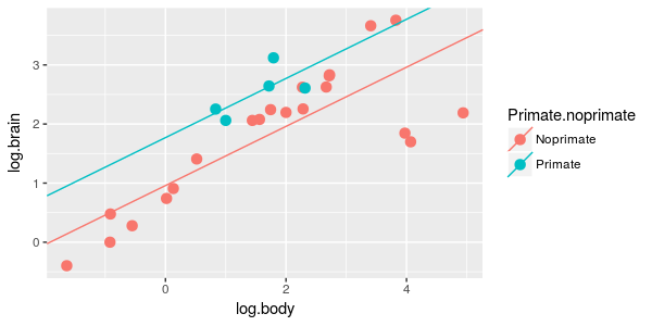
| 6. Brain/body scaling is the same for primates and non-primates, but with different averages between the groups. |
ANCOVA of log.brain by primate.noprimate, with log.body as a covariate
 |
What is the model? | primate.lm |
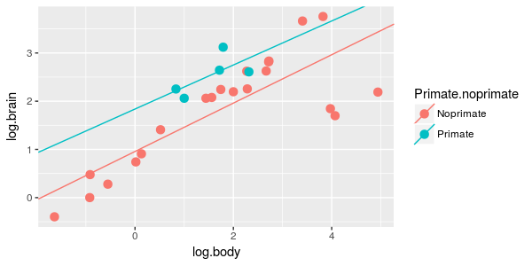
| 7. Brain/body scaling is different for primates and non-primates. |
ANCOVA of log.brain on primate.noprimate and log.body, with an interaction between primate.noprimate and log.body
 |
What is the model? | primate.int.lm |
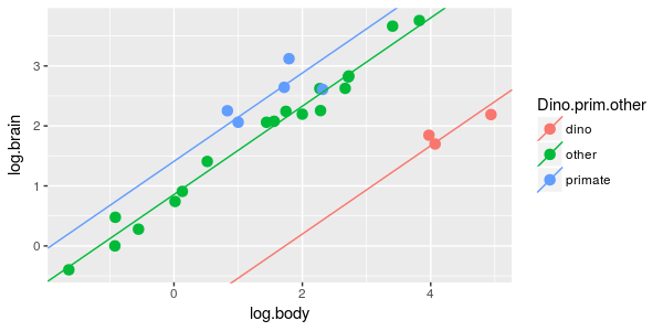
| 8. Brain/body scaling is the same for dinosaurs, primates, and other mammal, but with different averages between the groups. |
ANCOVA of log.brain by dino.prim.other, with log.body as a covariate
 |
What is the model? | dpo.lm |
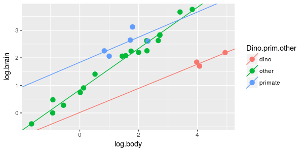
| 9. Brain/body scaling is different for dinosaurs, primates, and other mammals. |
ANCOVA of log.brain on dino.prim.other and log.body, with an interaction between dino.prim.other and log.body
 |
What is the model? | dpo.int.lm |
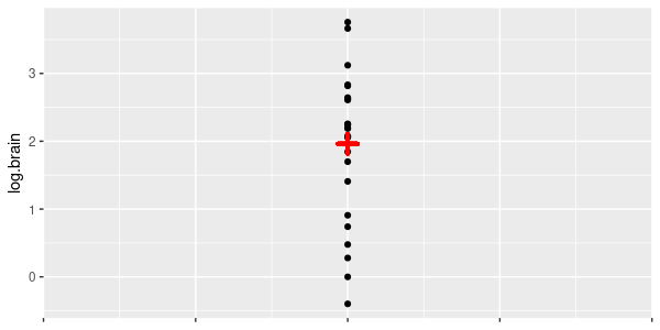
| 10. There is no predictable relationship between brain size and body size for these species. In other words, brain size is independent of body size. |
The "intercept only" model.
 |
log.brain ~ 1 | intercept.only.lm |
When you're done you can check the names in your list (in the show.model.list.elements chunk of the Rmd file):
names(models.list)
You should see the names:
[1] "body.lm" "taxa.lm"
"taxa.int.lm" "dino.lm"
[5] "dino.int.lm" "primate.lm" "primate.int.lm"
"dpo.lm"
[9] "dpo.int.lm" "intercept.only.lm"
If you don't see this list of names, read the blockquote section for instructions for fixing errors.
IF YOU MAKE A MISTAKE read this for the fix (otherwise skip to step 2 below).
- If you made a mistake in the model statement, but used the correct model name, edit the command and assign the correct model to the same named list element. The mistake will be replaced by the corrected model.
- If you use the right model statement but used the wrong model name, you can change the name if you know the number of the model. Look at the number of the named elements, and find the number for the incorrect one. For example, if you were to get names like:
[1] "boody.lm" "taxa.lm" "taxa.int.lm" "dino.lm"
[5] "dino.int.lm" "primate.lm" "primate.int.lm" "dpo.lm"
[9] "dpo.int.lm" "intercept.only.lm"
The incorrect name is the first in the list, which has index number 1. You can change its name with:
names(models.list)[1] <- "body.lm"
This will replace the wrong name with the right one.- If you accidentally included a model that you don't want, use the command:
models.list$mistake.name <- NULL
This will delete the model from the list.
2. Get the AIC statistics. After you have added all 10 models to models.list you need to extract their AIC values for analysis. We can use sapply() for this, using R's extractAIC() function applied to each of the named models in models.list.
Note that we could use the glance() function again, like we did for the adjusted R2-based model selection exercise we did a couple of weeks ago, but we'll use a different approach here because it makes makes some of the calculations a little easier.
The extractAIC() function extracts AIC and number of parameters from a fitted model. Try it out in the Console on the first model, body.lm, with the command (in the console):
extractAIC(models.list$body.lm)
You will get two values, the first being the number of parameters in the model (K in the AIC formula, equal to 2 for this model), and AIC (which is -17.36706 for this model).
We can use extractAIC() as the function in an sapply() command, which will extract K and AIC for each model in models.list. The command is (in the Console):
sapply(models.list, extractAIC)
which gives you this:
body.lm taxa.lm taxa.int.lm dino.lm dino.int.lm primate.lm primate.int.lm dpo.lm
[1,] 2.00000 8.00000 14.00000 3.00000 4.00000
3.00000 4.0000 4.00000
[2,] -17.36705 -79.14906 -70.07542 -58.16365 -56.81901 -22.22915 -20.2379 -76.33646
dpo.int.lm intercept.only.lm
[1,] 6.000 1.000000
[2,] -77.238 4.424834
This command gives us the information that we want, but it's in the wrong orientation - each model is a column instead of a row, and our numbers of parameters and AIC's are rows instead of columns. Fortunately, swapping rows and columns is a simple matrix operation called "transposition". We can transpose the matrix using the t() command (in the Console):
t(sapply(models.list, extractAIC))
which gives us:
[,1] [,2]
body.lm 2 -17.367054
taxa.lm 8 -79.149058
taxa.int.lm 14 -70.075416
dino.lm 3 -58.163652
dino.int.lm 4 -56.819013
primate.lm 3 -22.229149
primate.int.lm 4 -20.237899
dpo.lm 4 -76.336462
dpo.int.lm 6 -77.237999
intercept.only.lm 1 4.424834
This output has the orientation we want, so we're almost there. At this point the output is still a matrix rather than a data frame, which we can fix by wrapping our t(sapply()) inside of a data.frame() command, like so (put this version into the extract.aic chunk of your Rmd file):
model.aic <- data.frame(t(sapply(models.list, extractAIC)))
If you type model.aic you'll see you now have the data organized as we want, but without informative column names. We can add column names to the model.aic data frame with (in the rename.k.and.aic.columns chunk of your Rmd file):
colnames(model.aic) <- c("K","AIC")
The final version of the table, with column labels, looks like this:
K AIC
body.lm 2 -17.367054
taxa.lm 8 -79.149058
taxa.int.lm 14 -70.075416
dino.lm 3 -58.163652
dino.int.lm 4 -56.819013
primate.lm 3 -22.229149
primate.int.lm 4 -20.237899
dpo.lm 4 -76.336462
dpo.int.lm 6 -77.237999
intercept.only.lm 1 4.424834
The list of model names on the left are row names for the data frame rather than a column of data, so they do not have a column name.
3. Calculate AICc. Now that we have K and AIC for each model in our model.aic data frame, we can calculate AICc. AICc is just AIC plus an additional penalty for each model parameter, equal to 2k(k+1)/(n-k-1). k will come from the K column of model.aic, and n is the sample size (which is 26 for this data set).
In the console you can see what the calculation will look like with this command:
with(model.aic, AIC + 2*K*(K+1)/(26-K-1))
This will give you an AICc value for each of the models, like so:
[1] -16.845315 -70.678470 -31.893598 -57.072743 -54.914251 -21.138240 -18.333137
[8] -74.431700 -72.816947 4.591501
This worked fine, but to enter n we have to look at the number of observations in brains (26) and enter the number. We can make this unnecessary by using nrow(brains) to get the number of observations for us. The final calculation is thus (in the calculate.AICc chunk of your Rmd file):
model.aic$AICc <- with(model.aic, AIC + 2*K*(K+1)/(nrow(brains)-K-1))
If you type model.aic, you'll see there is now a column called AICc with the results of these calculations.
4. Calculate delta AICc. We can now calculate delta AICc values, which are much easier to interpret than the raw AICc values. The command is (in the calculate.delta.AICc chunk of the Rmd file):
model.aic$dAICc <- model.aic$AICc - min(model.aic$AICc)
This command takes the AICc's we just calculated and subtracts the smallest AICc from each of them. Type model.aic in the console and you'll see:
K
AIC AICc dAICc
body.lm 2 -17.367054 -16.845315 57.586385
taxa.lm 8 -79.149058 -70.678470 3.753230
taxa.int.lm 14 -70.075416 -31.893598 42.538102
dino.lm 3 -58.163652 -57.072743 17.358957
dino.int.lm 4 -56.819013 -54.914251 19.517449
primate.lm 3 -22.229149 -21.138240 53.293460
primate.int.lm 4 -20.237899 -18.333137 56.098563
dpo.lm 4 -76.336462 -74.431700 0.000000
dpo.int.lm 6 -77.237999 -72.816947 1.614753
intercept.only.lm 1 4.424834 4.591501 79.023201
The model with the smallest AICc has a dAICc of zero, and the rest are differences from this model's AICc.
5. Calculate the weights, w. Finally, let's calculate the Akaike weights. Remember, these are measures of how often we would expect the model to be best-supported if we repeated the exercise with new data; they are useful for attaching a more intuitive interpretation for degree of support for the models than we get from the ΔAICc values alone. These are calculated with (in the calculate.AICc.weights chunk of your Rmd file):
model.aic$wts <- with(model.aic, exp(-dAICc/2)/sum(exp(-dAICc/2)))
This calculation divides each model's exp(-dAICc/2) by the sum of the exp(-dAICc/2) for all of the models. Dividing a part by a total always gives us proportions, so these values will fall between 0 and 1, and sum to 1 across the models.
6. Sort the table on dAICc. Traditionally, tables of AIC statistics are sorted on dAICc to make it easier to see which models are best supported. We're going to use the order() command to give the rank order of the dAICc values - in the console write:
order(model.aic$dAICc)
and you will get:
[1] 8 9 2 4 5 3 6 7 1 10
After the index, [1], the numbers are the row numbers from dAICc - the eight row is the smallest dAICc, the ninth is the second smallest dAICc, and so on. We can use these numbers to sort the entire model.aic data frame if we use them as the row index - do so with this command (in the console):
model.aic[order(model.aic$dAICc), ]
which gives you:
K
AIC AICc dAICc wts
dpo.lm 4 -76.336462 -74.431700 0.000000 6.252494e-01
dpo.int.lm 6 -77.237999 -72.816947 1.614753 2.788778e-01
taxa.lm 8 -79.149058 -70.678470 3.753230 9.573036e-02
dino.lm 3 -58.163652 -57.072743 17.358957 1.063172e-04
dino.int.lm 4 -56.819013 -54.914251 19.517449 3.613209e-05
taxa.int.lm 14 -70.075416 -31.893598 42.538102 3.622611e-10
primate.lm 3 -22.229149 -21.138240 53.293460 1.673113e-12
primate.int.lm 4 -20.237899 -18.333137 56.098563 4.115334e-13
body.lm 2 -17.367054 -16.845315 57.586385 1.955819e-13
intercept.only.lm 1 4.424834 4.591501 79.023201 4.328956e-18
This command put the row numbers from the order() command into the row index position for model.aic, which puts the model.aic data in order by the dAICc column.
We can compare the weights more easily if we suppress the scientific notation - use the command (in your Rmd file, sort.and.display.output chunk):
format(model.aic[order(model.aic$dAICc),], digits = 2, scientific = F)
which gives you:
K AIC AICc
dAICc wts
dpo.lm 4 -76.3 -74.4 0.0 0.6252493597029067374
dpo.int.lm 6 -77.2 -72.8 1.6 0.2788778324035202094
taxa.lm 8 -79.1 -70.7 3.8 0.0957303581929313807
dino.lm 3 -58.2 -57.1 17.4 0.0001063172432656724
dino.int.lm 4 -56.8 -54.9 19.5 0.0000361320928347135
taxa.int.lm 14 -70.1 -31.9 42.5 0.0000000003622611060
primate.lm 3 -22.2 -21.1 53.3 0.0000000000016731133
primate.int.lm 4 -20.2 -18.3 56.1 0.0000000000004115334
body.lm 2 -17.4 -16.8 57.6 0.0000000000001955819
intercept.only.lm 1 4.4 4.6 79.0 0.0000000000000000043
As you interpret this table, remember:
- The best-supported model has the lowest AICc, and will have a dAICc of 0
- dAICc values below 2 are considered more or less equivalent models - they are both well supported by the data, and the data provides little basis for preferring one over the other
- dAICc values of 4 to 10 indicate substantially lower support than the best supported model
- dAICc values over 10 are sufficiently large that the models can be disregarded
You should see that the weight is biggest for the model with a dAICc of 0, but for models with dAICc's less than 4 the weights are still fairly high. Based on these weights we can be confident that some hypotheses are very poorly supported by the data (intercept.only.lm, body.lm, and the other models with dAICc above 10), but there are three with dAICc values less than 4 (taxa.lm, dpo.int.lm, and dpo.lm), one of which has a dAICc of only 1.6. With these data we do not have enough support to just interpret the best-supported model, and should consider dpo.int.lm as fairly equivalent to dpo.lm. The taxa.lm model has substantially less support than either dpo.int.lm or dpo.lm, but with a weight slightly below 4 it cannot be completely discounted.
7. Interpretation of variables. At this point we have information about how much support there is for each model in the data, but that's only the first step in data analysis. We can address how important individual variables are by summing the weights for the models each variable appears in. There are various ways of doing this, but the seemingly simplest method of calculating them by hand is error-prone, and it would be much better to take advantage of the fact that we already have the information we need in the models.list and model.aic objects. We just need to figure out how to get it in a form that can be used to calculate the weights by variable.
To do this calculation, we will:
- Make a data frame with variable names as columns, and model names as rows.
- Multiply the matrix of 0's and 1's by the model weights to get the weight for each model a variable occurs in into its column
- Sum the columns
The data frame we want to make looks like this:
log.body Taxa Dino.nodino Primate.noprimate Dino.prim.other
body.lm 1 0
0 0 0
taxa.lm 1 1
0 0 0
taxa.int.lm 1 1
0 0 0
dino.lm 1 0
1 0 0
dino.int.lm 1 0
1 0 0
primate.lm 1 0
0 1 0
primate.int.lm 1 0
0 1 0
dpo.lm 1
0 0
0 1
dpo.int.lm 1 0
0 0 1
intercept.only.lm 0 0
0 0 0
To make this table, we start with a vector that has the names of the predictor variables, which will end up being the columns in the table - in chunk which.models.variables.are.in enter:
predictors <- c("log.body","Taxa","Dino.nodino","Primate.noprimate","Dino.prim.other")
The next thing we want to do is to compare the predictor variables used in each model to this set, so we need to extract the variables used in the models. For example, we can get the names of the predictors in dpo.int.lm with (in the console):
all.vars(formula(models.list$dpo.int.lm))
This gives us the response variable first, followed by the two predictors. Now to get the row of the matrix we're building for model dpo.int.lm we would want to see if each of the predictor variables in predictors is in this set of two predictors we used in dpo.int.lm, like so (in the console):
predictors %in% all.vars(formula(models.list$dpo.int.lm))
you should see the output:
[1] TRUE FALSE FALSE FALSE TRUE
These are in the order that we entered the predictor variables in predictors, so the first TRUE is for log.body, and the final one is for Dino.prim.other. The FALSE entries indicate that the rest of the predictors do not appear in the predictor variables in dpo.int.lm.
Okay, now we have the basic procedure, we just need to apply this to each model in models.list, and output the results as a matrix. In the console enter:
sapply(models.list, FUN = function(x) predictors %in% all.vars(formula(x)))
This gives us the matrix we need, but with a couple of issues: the variable names aren't included, and the table is laid out wide instead of long. We can fix all of those with this final version - in the code chunk which.models.variables.are.in below the predictors list, enter:
data.frame(t(sapply(models.list, FUN = function(x) predictors %in% all.vars(formula(x))))) -> variables.in.model
colnames(variables.in.model) <- predictors
The final version of the sapply() function still has the results in the form of TRUE and FALSE instead of 1 and 0, but that's not a problem because TRUE and FALSE are usable as the numbers 1 and 0 in calculations - if we wanted to we could use as.numeric(variables.in.model) to convert to 1 and 0, but it's really not needed. The orientation of the matrix was fixed using t(), and then it was converted to a data.frame(). Once variables.in.model was created, the names of the predictors could be assigned as column names.
Now that we have the variables.in.model data frame, we can use it to select which model weights to include when calculating the importance for each variable. If we multiply the model weights by each column in the variables.in.matrix data frame, we'll get the weight everywhere we have a 1, and a 0 everywhere we have a 0. In the console type:
model.aic$wts * variables.in.model
to get:
log.body Taxa Dino.nodino Primate.noprimate Dino.prim.other
body.lm 1.955819e-13 0.000000e+00 0.000000e+00 0.000000e+00
0.0000000
taxa.lm 9.573036e-02 9.573036e-02 0.000000e+00 0.000000e+00
0.0000000
taxa.int.lm 3.622611e-10 3.622611e-10 0.000000e+00 0.000000e+00 0.0000000
dino.lm 1.063172e-04 0.000000e+00 1.063172e-04 0.000000e+00
0.0000000
dino.int.lm 3.613209e-05 0.000000e+00 3.613209e-05 0.000000e+00 0.0000000
primate.lm 1.673113e-12 0.000000e+00 0.000000e+00 1.673113e-12 0.0000000
primate.int.lm 4.115334e-13 0.000000e+00 0.000000e+00 4.115334e-13 0.0000000
dpo.lm 6.252494e-01 0.000000e+00 0.000000e+00 0.000000e+00
0.6252494
dpo.int.lm 2.788778e-01 0.000000e+00 0.000000e+00 0.000000e+00 0.2788778
intercept.only.lm 0.000000e+00 0.000000e+00 0.000000e+00 0.000000e+00 0.0000000
Each number in the output is now either the weight for the model (if a variable occurred in it), or a 0 (if the variable did not occur in it). This means that every column has the weight for every model a variable occurs in, and we can just sum the columns to get a measure of how important the variable is.
To do this, change the last command to (in the console):
colSums(model.aic$wts * preds.by.model)
and you will see:
log.body Taxa
Dino.nodino Primate.noprimate Dino.prim.other
1.000000e+00 9.573036e-02 1.424493e-04
2.084647e-12 9.041272e-01
These values too fall between 0 and 1 - the closer to 1 they are the more important the variable is to include, and the better supported it is by the data.
These variable importance values are complete, but are a little hard to compare because of the scientific notation. So, for the final command for the calculate.variable.weights chunk of your Rmd file should use the format() command to suppress scientific notation:
format(colSums(model.aic$wts * variables.in.model), scientific = F)
you'll see:
log.body Taxa
Dino.nodino Primate.noprimate Dino.prim.other
"1.000000000000000000" "0.095730358555192491" "0.000142449336100386" "0.000000000002084647" "0.904127192106426891"
What can we learn from these? At the level of the models, we had nearly the same support for dpo.lm and dpo.int.lm, which had a dAICc of only 1.6, which left us unsure which model was the best. Based on these variable weights we can be very confident that Dino.prim.other and log.body are both very important predictor variables, even though the importance of the interaction between them is less certain. The sum of the weights for the nine models that include log.body is very close to 1, and the sum of the weights for the two models that include Dino.prim.other is 0.904. We may not be sure whether the groups have the same slope to their lines or not, but we can be quite confident that the best grouping of the taxa separates dinosaurs and primates, but keeps the rest of the mammals lumped together.
Taxa is interesting as a predictor variable, because it separates all of the taxa, which means that it must also separate the dinosaurs, primates, and other mammals like Dino.prim.other does. Even if all the other mammals aren't different from one another, Taxa can represent this fact by having a bunch of intercepts that are the same for all the mammal Orders, aside from primates. This means that, while the dpo.lm model would predict identical brain sizes for an artiodactyl and a carnivore that had the same weight, Taxa have to estimate intercepts for artiodactyls and carnivores, even if they were nearly identical values. Splitting the different mammalian Orders in the Taxa predictor would end up adding a bunch of additional coefficients without explaining much extra variation, and the penalty for complexity wipes out any gains in logLikelihood when the AICc is calculated. The trade-off between complexity and fit is working against Taxa compared with Dino.prim.other.
Note one more quirk of the way that I've designed this analysis - log.body is in every model except for the intercept only model. Not surprisingly, its importance is near 1, because we haven't really made it compete against other hypotheses in which it was omitted. The reason I did this was to focus on the matter of which taxonomic grouping was best supported, and we took it as a given that there was a brain size/body size relationship. If we seriously thought that there might not be a relationship between brain size and body size at all then this would be a bad thing to do - instead we should have models that have the grouping variables without log.body included to assess the possibility that the different groupings of taxa are all we needed to understand differences in brain size, and that knowing the body size added nothing to our understanding. Essentially, by structuring the analysis the way I did we took as a given that bigger animals should have bigger brains, and we focused only on which taxonomic grouping added the most to our understanding. The point is not that this was either a correct or incorrect choice, but just consider that your choices of models affect what you can learn from the analysis.
Rethinking post-hocs from a Method of Support perspective
There's nothing wrong with the usual questions we ask with an analysis like ANCOVA. Wanting to know the relationship between brain and body weight, and how groups of species differ in brain size at a common body weight, are perfectly good scientific questions to ask, and we don't need to abandon them to use the MOS.
To demonstrate this to you, I'll show you how we can use the MOS to reproduce the typical ANCOVA analysis, complete with an equivalent to post-hoc comparisons between groups of the categorical predictor.
For example, if we were only interested in a single categorical predictor, Dino.prim.other, in a conventional ANCOVA, we would test if the model including Dino.prim.other and log.body was significant, and if the Dino.prim.other effect was significant we would need to conduct post-hocs to see which of the three groups were different from one another. We can reproduce this approach using model selection, without any null hypothesis significance tests.
First, we would want to do the equivalent of a test of the null hypothesis for the overall ANCOVA model. We could do this by fitting the intercept-only model and dpo.lm, and seeing which was best supported. We have these two models in the analysis we already completed, and their AICc statistics are:
K AIC AICc dAICc
dpo.lm 4 -76.336462 -74.431700 0.0000
intercept.only.lm 1 4.424834 4.591501 79.0232Clearly accounting for log.body and Dino.prim.other is well supported. But, this doesn't isolate the effects of Dino.prim.other from log.body, the way an ANCOVA table would. We can do that, though, by including body.lm as one of the models in our AICc table:
K AIC AICc dAICc
dpo.lm 4 -76.336462 -74.431700 0.00000
body.lm 2 -17.367054 -16.845315 57.58639
intercept.only.lm 1 4.424834 4.591501 79.02320
The model with log.body alone is much better supported than the one with only an intercept (79.02 - 57.48 = 21.54), but accounting for groupings for dinosaurs, primates, and other mammals in this brain/body relationship is even better supported. Since the only difference between body.lm and dpo.lm is the Dino.prim.other variable, this is good evidence that dinosaurs, primates, and other mammals have different average brain sizes after accounting for any differences in body mass.
Note that this approach treats the null hypothesis as just another hypothesis, no different from the hypotheses about the existence of a relationship between predictors and response. This gets away from the false dichotomies that arise from testing only a null hypothesis for significance, while letting us retain the very important hypothesis of no relationship whatsoever between the variables in our analysis.
Having gotten this far with an ANCOVA we would also want to know which of the three groups are different from one another. With a conventional ANCOVA analysis we would address this with Tukey post-hocs, and then afterward might use something like the compact letter display to determine what the "homogeneous subsets" are - that is, which groups are not different from one another and which are. We can use the MOS to find the homogeneous subsets as well, but we do it using a set of models that have either lumped together or split apart the three categories of Dino.prim.other.
The possible homogeneous groupings are as follows:
If you look these over you'll see that one of possible re-grouping missing: the combination of primates and dinosaurs in one group, with other mammals separated into another. We could make this model easily enough, but it doesn't really make sense as a hypothesis - the brain sizes from largest to smallest are primate, other mammals, dinosaurs, and it makes sense to ask whether ones that are next to each might not actually be different, but it doesn't make sense to group the mammals (largest) and dinosaurs (smallest) and keep the other mammals separate. We aren't obligated to consider silly hypotheses, and a thoughtful process is better than a blind, exhaustive search through the possibilities.
So, we need a model for each of these four possible groupings. As it happens, we already have them:
- All three groups are hypothesized to be the same by the body.lm model (right? Omitting a predictor hypothesizes the groups are all the same)
- Dinosaurs are hypothesized to be different from all of the mammals, but primates and other mammals are grouped together, in the dino.lm model
- Primates are separated, but the rest of the mammals and the dinosaurs are grouped in the primate.lm model
- All three are separate in the dpo.lm model
We can extract the stats for these models from the model.aic table like so (in the console):
model.aic[ c("body.lm","dino.lm","primate.lm","dpo.lm"),c("K","AICc","dAICc")]
which gives you:
K AICc dAICc
body.lm 2 -16.84531 57.58639
dino.lm 3 -57.07274 17.35896
primate.lm 3 -21.13824 53.29346
dpo.lm 4 -74.43170 0.00000Based on this table, the dpo.lm model has much lower AICc than the next closest grouping. The second best supported model is dino.lm, but with a dAICc of 17.35 we can disregard it and just interpret dpo.lm alone, without having to consider any other possible groupings.
Given this, separating all three categories is by far the best-supported option, and we can take this as evidence that all three groups of species are different from one another in their average brain sizes. This answers the question we would usually address using Tukey post-hocs - we have evidence that the three groups are different, but we generated no p-values to reach that conclusion.
8. Check the assumptions of GLM for any models you want to interpret. Using model selection doesn't relieve us of the responsibility to make sure that our model fits the data. Ultimately it only really matters that the models we interpret meet GLM assumptions, so we will focus on dpo.lm and dpo.int.lm. In the chunk check.assumptions of your Rmd file enter:
par(oma = c(0,0,3,0), mfrow = c(2,2))
plot(models.list$dpo.lm)
plot(models.list$dpo.int.lm)
You'll see that the residual plots look really good - these models fit well.
We don't need to worry about whether poorly supported models meet GLM assumptions, because one of the reasons they might fail to do so is that they don't include the right predictors, and
that is already accounted for when we compare AICc values. For example, the body.lm model might not meet GLM assumptions because we're not accounting for any groupings in the data, but this is also a reason why body.lm has such a high dAICc. For the models we do want to
interpret we should confirm we are meeting the assumptions of our linear models so that we know that our interpretations will be accurate.
because we're not accounting for any groupings in the data, but this is also a reason why body.lm has such a high dAICc. For the models we do want to
interpret we should confirm we are meeting the assumptions of our linear models so that we know that our interpretations will be accurate.
9. Get the model R2. One last thing before we put too much confidence in our best-supported models is: we need to stop and remember that "best supported" is a relative term, and can only ever pertain to the models we've included in the analysis. With our analysis of brain sizes, all we have done so far is to establish that models that include the dpo predictor along with log.body are well supported compared to models that use other groupings of the taxa. But, it could be that dpo.lm and dpo.int.lm are just the best of ten terrible models.
For example, we could get big differences in AICc between models with multiple R2 of 0.1, 0.01, 0.001, or 0 (with 0 for the R2 of the intercept-only model), but the best of this sorry bunch still only explains 10% of the variation in the response and should not be the basis for any firm conclusions about what determines brain size. We do not have a large sample size here, but the point is even more important with larger data sets, because the amount of difference btween the AICc values gets bigger for a given effect size with larger sample sizes.
So, in addition to dAiCc and model weights, we should always have a measure of how well the model explains variation in the response variable, such as the R2. We can extract the multiple R2 for each of the models with (in the extract.r.squared chunk of the Rmd file):
sapply(models.list, FUN = function(x) summary(x)$r.squared)
You should see the following:
body.lm taxa.lm
taxa.int.lm dino.lm dino.int.lm
0.5995125 0.9765490
0.9790453 0.9227799 0.9247020
primate.lm primate.int.lm
dpo.lm dpo.int.lm intercept.only.lm
0.6924136 0.6925171
0.9644556 0.9705627 0.0000000
Aside from the intercept only model, which explains no variation in the response at all and will always have an R2 of 0, all of the other models have R2 of 0.6 or higher. The best-supported models have values of 0.96 or 0.97, which are close to perfect. From this we can conclude that the best supported models are also very good models of variation in brain size for these species.
What more do you want to know?
We won't be taking the interpretation of our models any further today for lack of time, but if we did, all of the interpretation steps we have used all semester are still appropriate here. For example, our models are ANCOVA's, so for the best supported models we could:
-
Use least squares means to get body mass-adjusted brain sizes across the levels of the dpo categorical variable, for dpo.lm
-
Compare the slopes across the categories for dpo.int.lm
That's it! Knit and upload your Word file and you're all done. Next stop, final exam!