Who should be using this version of the simulation
I had a student tell me he had some experience with R, and was hoping
to learn more about it in Biol 365. I offered to make a version of the
simulation modeling exercise that uses R instead of Excel for him, as
well as for anyone who has had enough Excel, and wants to expand their R
skills.
Given that, I wrote this to work for a student who knows some R
already. If that isn't you, then I strongly recommend that you do the
Excel version of the assignment, because these instructions will be hard
to understand if you have never used R before. If you're really sick of
Excel, and are up for a challenge, then you're welcome to give it a try,
but expect a much steeper learning curve than if you stick with Excel.
Introduction to the assignment
For the final three weeks of class, you will build a simulation model
of genetic drift. Genetic drift is important to evolutionary biology,
plant and animal breeding, biotechnology, and biological conservation.
We will focus on the conservation applications in this case, and as such
we will focus on how genetic drift affects allelic diversity (which is
important for a species' ability to adapt to its environment) and
heterozygosity (which is important for avoiding genetic disorders, and
for an individual's ability to fight off wide ranges of infectious
diseases).
We will break the work down into four stages:
Initial setup of the populations, and simulation of a single run of
500 generations. This is your goal for this week.
Modification to run the simulation 100 times, collect data from
each. This is the goal for next Monday.
Increase population size
Add immigration. These last two are easy, and can both be done on
the last day or two of class.
You should be able to complete these four versions of the model by the
end of the final day of class, on May 6th. When you've completed the
simulations you will write up the results and submit your writeup and
simulation models in place of a final exam for the class.
Software and R Markdown files
I assume that you already know something about R, but briefly... R is a
an open source programming language and statistical analysis
environment. "Open source" is a software development method, in which
the programming code is available for anyone who wants to look at it,
and allows contributions of features and bug fixes from users. Open
source software development was devised by advocates of "free software",
which is a movement based around the rights of users, including the
right to inspect the code for the programs they use (since "free" in
English can pertain either to speech or beer, free software is often
called "libre software" to clarify that advocates are referring to free
in the sense of freedom, not in the sense of a price equal to zero).
This openness tends to lead to a couple of nice things: first, the
software is usually distributed for free, because anyone who knows how
could compile the freely-available code any time they wanted to. Second,
because so much is being given away for free, R users tend to be
grateful, and to contribute extension "libraries" that greatly expand
the capabilities of R. There are more than 10,000 user-contributed
packages available, and some have been nearly indispensable (the R
developers don't feel much urgency about implementing things that are
readily available as contributed libraries).
These instructions assume you will be using the R Studio integrated
development environment. It is on the student computer lab machines, but
you can also download it to install on your own computer from here
(it is also free). Follow the installation instructions, as you have to
install R first.
Once you have R Studio installed, start it and make a new project for
the simulation model - do this with File → New Project... ; use the "New
Directory" option to make a new folder for the project and all its
files. Call the project "drift_simulation" (the underscore is a good
idea, as it's easier to use R when there are no spaces in names of
things).
When you're done you'll see in the "Files" tab that there is a file
called drift_simulation.Rproj, which is the "project file" created when
you made the new project. R Studio uses this file to keep track of
things like the sizes of the four panels of the R Studio window, whether
you have any files open, and so forth.
By far the easiest way to use R within R Studio for class projects like
this one is to write documents with R Markdown, which is a format that
allows you to mix text explanations with executable "code chunks" where
you can run commands. I have prepared an Rmd file for you to use for
this exercise, with code chunks for all of the steps you need to
complete. The file for the first two stages of the simulation is called
step1_and_2_setup_and_run_n100.Rmd - download it and move it into
your new project folder. When it's in the project folder you'll see it
in the "Files" tab in R Studio, so click on it there to open it (DO NOT
click on it in the Downloads folder and start working on it from there,
you really want to have it in the project folder to avoid issues later).
A code chunk is created using a line with an opening set of characters,
followed by one or more blank lines, and then another line with closing
characters, like so:
The opening line is:
```{r make.parent.male.pop}
It is formed using three "back-ticks" (on the key to the left of the 1
on the keyboard) followed by curly brackets with the code word "r"
inside of them, {r}. Optionally, you can add a label, which every one of
the code chunks I've given you will have - this one is labeled
"make.parent.male.pop", and this is how I will direct you to the right
code chunk to enter the commands below. Just match the label I specify
in the instructions below with the label in the brackets and everything
should work fine.
If you look in the upper right corner of the code chunk, there is a
"run" button, which is a right-pointing green triangle. When you have
your code entered you click the "Run" button to run it.
Okay, with that very brief intro, you can get started.
Stage 1: Setting up the simulation model
The model will be general, and is not meant to model a particular
species. However, we have some choices to make about how to construct
the simulation that need to be guided by biological characteristics. So,
in a general sense, the "species" we are simulating will have the
following properties:
Diploid (meaning there are two alleles per gene, one inherited from
the mother and one from the father)
Sexually reproducing
Random mating
The model will be individual-based (meaning that our
model will simulate individuals in the population), and will be a simulation
model (meaning that we will study the virtual individuals to
understand how drift affects the gene pool rather than writing equations
and finding the solutions for particular variables). Random changes in
gene frequency (i.e. genetic drift) will emerge from the process of
random mating between our simulated individuals, which will randomly
select some individuals to produce offspring while others produce none.
The fact that mates will be selected at random from the population will
make the model stochastic, and each simulation run
will be somewhat different from any other. Our model will thus be a stochastic
individual-based simulation model.
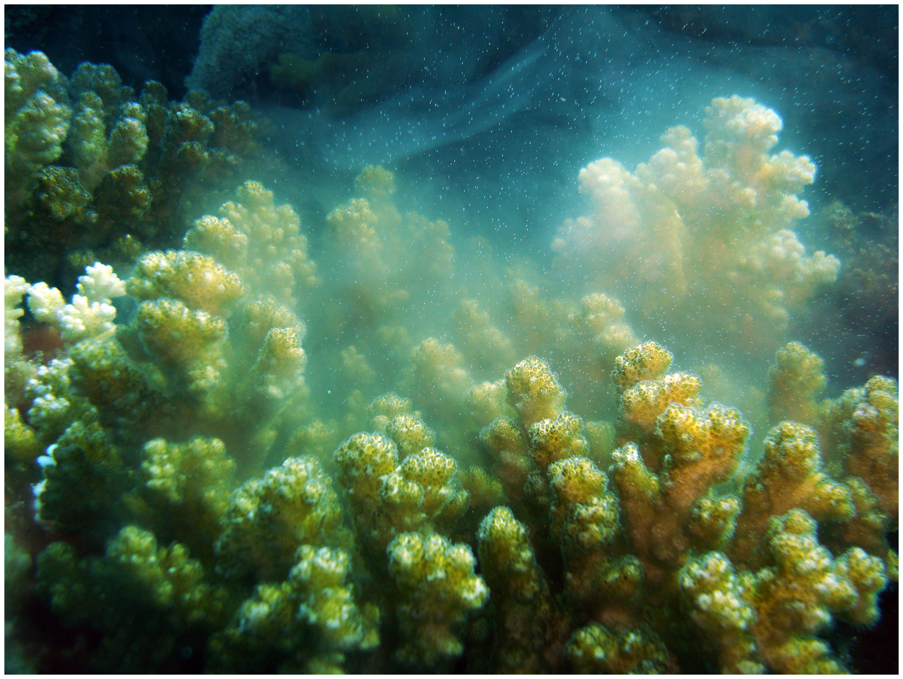
Although we don't need to specify a particular species that our model
represents, the type of random mating we will simulate is easiest to
imagine from "broadcast spawning", which is common in
attached marine invertebrates like the coral polyps in the example
image. Species such as anemones are not capable of moving around to find
a mate, and both males and females release their gametes into the water
column, where fertilization occurs. There is little opportunity in
broadcast spawning for individuals to select mates, and random mixing of
alleles is the best model of how it works.
To keep the simulation relatively simple we will only concern
ourselves with a single gene with 5 different alleles. Any single
individual can only have two alleles, one of which was inherited from
its mother and one from its father, but different individuals in a
population can have different ones - the five alleles in the population
will be labeled A, B, C, D, and E.
The first thing we need to do is to establish our initial populations
of individuals. We will only use two properties of each individual: sex
and genotype.
Step 1. Set up initial parent
population.
We need to set up the genotypes for the parent population, which will
establish the starting allele frequencies for the population's gene
pool. We'll refer to these as the initial conditions,
and each time we run the simulation we'll return the population to this
starting point. First we'll set up the layout.
Open R Studio and start a new
project. Make a new folder to keep everything nice and organized.
Step 2. Initial conditions:
establish the genotypes of the first 100 individuals in the population
We will begin this population all five of the alleles (A, B, C, D, and
E) at a frequency of 0.2, which means that each of the five will
represent 20% of the total alleles in the population.
We can translate gene frequencies into genotype frequencies using the
Hardy-Weinberg formula. Hardy-Weinberg translates allele frequencies
into genotype frequencies by assuming that alleles combine at random, in
proportion to their frequencies in the population. We can see how it
works using a version of a Punnett square, with each parental allele in
a row and column label, which then combine to form genotypes of
offspring:
A
(0.2)
B
(0.2)
C
(0.2)
D
(0.2)
E
(0.2)
A (0.2)
AA
(0.22)
AB
(0.2)(0.2)
AC
(0.2)(0.2)
AC
(0.2)(0.2)
AE
(0.2)(0.2)
B (0.2)
AB
(0.2)(0.2)
BB
(0.22)
BC
(0.2)(0.2)
BD
(0.2)(0.2)
BE
(0.2)(0.2)
C (0.2)
AC
(0.2)(0.2)
BC
(0.2)(0.2)
CC
(0.22)
CD
(0.2)(0.2)
CE
(0.2)(0.2)
D (0.2)
AD
(0.2)(0.2)
BD
(0.2)(0.2)
CD
(0.2)(0.2)
DD
(0.22)
DE
(0.2)(0.2)
E (0.2)
AE
(0.2)(0.2)
BE
(0.2)(0.2)
CE
(0.2)(0.2)
DE
(0.2)(0.2)
EE
(0.22)
Homozygotes are produced when the same allele is contributed by each
parent, which means that if the frequency of the allele is p, then the
homozygous genotype should be produced at a frequency of p x p, or p2
- there is only one way in the table for each homozygous combination to
occur, so p2 is the final calculation of the frequency of the
genotype. Since all of the alleles have a frequency of 0.2, this means
homozygotes occur at a frequency of 0.04.
You can see that the Hardy-Weinberg values result from combining all
the alleles in the population with themselves, and since all of them
start with the same frequency in our model the frequencies of all the
combinations will all be the same at the beginning (that is, the
frequency of AA, BB, CC, DD, and EE will all start at 0.04).
A heterozygote with an A from their mother and a B from their father
has the same genotype as one who received a B from their mother and an A
from their father, so the fact that those heterozygous pairings happen
in two places in the table just means that their frequency will be pq +
qp, or 2pq.
We can thus get this simple initial set of frequencies in R using a
function called expand.grid() that makes every possible combination of
inputs. Let's make a vector with the allele names in it first, it will
come in handy in several places. In chunk make.parent.male.pop enter the
command:
alleles <- c("A","B","C","D","E")
You should see that an object called alleles is now in your environment
tab.
Below the alleles command, in the same chunk, you can use expand.grid()
to get all the possible combinations:
The expand.grid() function makes a new matrix with two columns, which
contain all of the combinations of values in the two vectors. Since we
used alleles twice as both vectors it produces all possible combinations
of the alleles A, B, C, D, and E, including alleles with themselves.
Each is placed in a different column of a data frame. The
"strings.as.factors = F" argument keeps the entries in the males data
frame as just characters, rather than "factors", which are a different
type of data in R. If you type males at the console you'll see that you
have 25 rows, and each row is a different genotype. Each homozygote
occurs once, and each heterozygote occurs twice, albeit with a different
order for the two (that is, A, B and B, A both appear).
We want to start with 50 males, not 25, so we can double the number of
males by selecting all 25 of the males twice, and then re-assigning the
full 50 of them back into the males data frame. In the same chunk, below
your expand.grid() command enter:
males[rep(1:25,2),] -> males
This replaces the version of males that had 25 rows with a new version
with 50. The way this is done is to use the command 1:25 to make a
sequence of numbers from 1 to 25, and then to repeat it twice. By
putting these numbers in the "row index" position, inside of square
brackets to the right of the name of the males data set, we get all 25
rows twice. The initial male population is set.
Why not just double males?
I'll put little "asides" that are not directly part of the work flow
into these gray boxes.
There are often multiple ways to do the same thing in R. Which to use
is often a matter of personal preference - for example, another way to
double the number of males would be to use the command:
rbind(males, males)
This works fine, so at this point it would be a perfectly good
alternative to the more complicated method of entering the row numbers
twice, as I had you do above.
But, the way that we did it is easier to use later in the simulation,
when we want to be able to vary the size of the population. R's
flexibility can make it a little harder to learn, but it gives you a
wide range of ways you can work, and you can pick the method that is
best for your particular needs.
The we should rename the columns to Allele1 and Allele2 for the sake of
clarity. Below the command you just completed, enter the command:
names(males) <- c("Allele1","Allele2")
If you type males in the Console you'll see the columns are now
renamed, and you have 50 rows.
The one thing that's still a little odd is that the row numbers go from
1 to 25, then start over at 1.1 and go to 25.1. We can fix this, and get
R to revert back to a sequential row number for every row, but entering
(below the names(males) command you just finished):
rownames(males) <- NULL
Now if you type males the row names are the same as the row number,
from 1 to 50.
3. Making the females is much simpler, because they have the exact same
initial setup as the males. In chunk make.parent.female.pop enter the
command:
females <- males
This makes a second copy of the males data frame with the same initial
conditions as the females.
Assignment operators
R allows you to use either arrows, -> or <-, or the equal sign,
=, as assignment operators. I have a mild preference for the arrows
(they're what I learned when I started using R), as they allow
assignment from either left to right (->) or right to left (<-),
and I like the flexibility. But, if you do use =, then it's equivalent
to <-, as it assigns whatever is entered on the right into the
object on the left of the equal sign.
Step 3. Measure the genetic
composition of the population
We will want to measure relevant characteristics of the population's
gene pool as the simulation progresses. There are several different
things we could measure, but the primary issues we would be interested
in from a conservation perspective are changes in numbers of alleles,
changes in their frequencies, and changes in heterozygosity.
The count of alleles is called allelic diversity. If
any allele goes to fixation that means it has reached
a frequency of 1, and is the only allele left in the population. This is
always the expected end result of genetic drift, given enough time, but
it can take longer under some circumstances than others. We are
interested in how long it takes to reach fixation, if it occurs over the
number of generations of random mating that we simulate. If a single
allele goes to fixation, all the others have gone to a frequency of 0
and are lost from the population. The allelic diversity is at its
minimum point when this happens.
We're also concerned about heterozygosity, which is
the proportion of individuals that are heterozygous for this gene. This
is also an important measure from a conservation perspective, and
although we know that it has to go to 0 if an allele reaches fixation
(since all individuals have to be homozygous if there is only one allele
in the population) it can decline to low levels before this happens. We
expect the highest levels of heterozygosity when the allele frequencies
are all the same, and as some alleles become more common (and others
necessarily become relatively less common) heterozygosity will decline
on average. It is possible for up to 100% of the individuals to be
heterozygous, and random mating can cause heterozygosity to increase
above what we would expect it to be, but on average we expect
heterozygosity to decline as the allele frequencies move away from equal
numbers.
1. First we will measure allelic
diversity. This is just a matter of counting up how many different
alleles are in the population. Initially we know this is 5, but it will
change as the simulation progresses, so we'll use the same method to get
the initial allelic diversity as we'll use at each step in the
simulation later.
There are several ways to do this, but we'll do it by first combining
the males and females into one data frame, and then using unlist() to
convert the two columns into one big vector of alleles.
In chunk combine.and.unlist.parent enter the command:
rbind(males, females) -> parents
Then use unlist to combine the two columns for Allele1 and Allele2 into
one big vector (next line, same chunk):
unlist(parents) -> parent.alleles
To count up how many alleles there are we first extract how many unique
letters are in this parent.alleles vector - in the count.unique.alleles
chunk:
unique(parent.alleles) -> parent.alleles.unique
Then we can count how many unique alleles there are using the length()
command - in the same chunk:
length(parent.alleles.unique)
You'll see there are 5 alleles at the beginning of the simulation, as
we already knew.
2. Next, we want to measure heterozygosity. We need to count up how
many heterozygous males or females there are and divide by the total
number of individuals.
Getting the number of heterozygotes is really simple, thanks to the
fact that "logical" data is interpreted as the values 0 and 1. If you
enter the command (in chunk heterozygosity):
sum(parents$Allele1 != parents$Allele2)
you should get a value of 20. This command is working by comparing the
entry in column Allele1 to the entry in column Allele2 for each
individual. The comparison is !=, which means "not equal to" (if we
wanted homozygotes we would use Allele1 == Allele2). Every time the two
alleles are different this comparison will return a TRUE, which is a
logical data type that is numerically equal to a 1. If the two alleles
are the same the comparison returns FALSE, which is equal to 0. Summing
these TRUE and FALSE values is the same as counting how many of the
alleles are different from one another.
To convert a count of how many individuals are heterozygous into a
heterozygosity we just divide by the number of individuals - edit your
command to be:
This should give you a value of 0.8, which is the correct value for the
initial heterozygosity.
3. Lastly, we will want to know the frequencies of all the alleles.
This too is simple once we created the parent.alleles object, we just
need to count up how many of each allele are present and divide by the
total.
In chunk allele.frequencies enter the command:
table(parent.alleles)
If you run this you'll see a table with counts of each allele. Edit
this command to divide by the total number of alleles:
table(parent.alleles)/length(parent.alleles)
You should see that all of the alleles start at a frequency of 0.2, in
a table that looks like this:
A B C
D E
0.2 0.2 0.2 0.2 0.2
We have one more issue to deal with that won't become a problem until
we start simulating drift over time, but if we set things up properly
now it will continue to work as the frequencies change. The issue is
that as alleles are lost we want their frequencies to go to 0, rather
than having them disappear from the table. For example, if by the end of
the simulation we have lost every allele but E we want the table to look
like this:
A B C
D E
0 0 0 0 1
instead of like this:
E
1
The reason this matters is that we'll be appending the frequencies on
to a results table, and for this to work well we need to have something
in every column of the table every time, even if it's a 0. We can make
this work, but first we have to convert parent.alleles into a "factor",
which is a type of variable in R that has "levels". If we specify the
levels when we convert to a factor it will keep all of them and count a
0 if it doesn't occur in the parent.alleles. Convert the command to:
Since we already made a list of alleles we can use it to specify the
levels in our factor() command. We aren't assigning this factor() output
to anything, so the only place the parent.alleles will be treated as a
factor is in this one command, without affecting any other (even the
length(parent.alleles) part of this command is using the un-converted
version of parent.alleles).
Again, it won't be an issue yet, but if we convert this output to a
matrix it will make appending this output to the results easier - edit
the command to read:
This is going to pay dividends later, even if the complexity doesn't
seem warranted yet.
Step 4. Set up the results
data.frame
1. Now that we have frequencies of all the alleles, heterozygosity,
and allelic diversity calculated for this initial generation, we need to
set up a place to record all of this information as each generation
passes. We can make a blank data frame called "results" by making a new
data frame with a column for each piece of information we want to
record, initialized to hold the numeric data that will go into it, but
with nothing entered yet. In chunk make.results.data.frame enter:
This will put a data frame called results in your environment, that
shows as having 0 observations of 7 variables.
2. Next, we should add the initial conditions to this data frame. We'll
need to go back and edit each of our commands to assign each result into
an object, then we'll be able to assemble them into a row of output and
append them to the results table.
Go back to count.unique.alleles and edit the command to read:
length(parent.alleles.unique) -> allelic
Next, go to the heterozygosity chunk and edit it to read:
Now to assemble these bits of output into something that can be
appended to the results table we just need to put them into a vector
together, in the order they appear in the results table. In chunk
bundle.output enter the command:
data.frame(t(freqs), hz, allelic)
If you run this you'll see you get a row of the values you've
calculated, in the same order they appear in the results table. The t()
command we're applying to the freqs means "transpose", and it converted
the column of frequencies into a row, which is what we needed here (this
is the payoff for using a matrix as the output for the frequencies
calculation).
Edit the command to assign into an object called initial.output (just
like you did for the others, assignment operator and then name of the
new object - give it a try).
Before we can append initial.output to results it needs to have the
same column names. As long as we're certain that the initial.output
values are in the same order as the results table, the simplest way to
do this is to take the names from results and assign them as names to
initial.output. In the bundle.output command, after the command that
creates initial.output, enter:
names(initial.output) <- names(results)
This works because the names() function can both report the names of an
object, and can accept input to change the names of an object. We are
getting the names of results, and then assigning them as the names for
initial.output.
Finally, we're ready to append the output to results - in chunk
add.initial.to.results enter:
rbind(results, initial.output) -> results
The rbind() function appends the second data frame (initial.output) to
the first (results). Putting initial.output second causes the intial
output to be appended - that it, it's added to the bottom of the
results. Since there's nothing it results it doesn't really matter, but
if we had reversed the order then initial.output would be added to the
top of the results table (prepending, instead of appending) - since
we're going to start simulating change over time we'll want to append
each generation's output to the end of the file, and we'll want to put
results first each time.
Simulate reproduction
The steps in simulating reproduction will be:
Randomly select the parents for each offspring (some parents will
have multiple offspring, some will have none)
Randomly select which of each parent's two alleles will get passed
on to the offspring they are producing
Make the offspring with the alleles selected from each parent
1. To randomly select the parents, we just need to generate random row
numbers and select the parents with those numbers to be the breeders.
The square brackets next to males are used to indicate rows and columns
(that is, the square brackets indicate males[rows, columns]). In the
rows position we're selecting 100 random numbers between 1 and 50, and
by using "replace = T" we're able to get the same number more than once
- this will mean that some males breed more than once, and some don't
breed at all. The column index position is left blank (notice the comma
with nothing after it before the closing bracket), which means that all
columns are being included for the selected rows.
We're going to produce 50 male and 50 female offspring each generation,
but we're selecting the fathers for them with this one command by
selecting 100 male breeders.
Do the same thing for females parents - assign into an object called
female.breeders.
2. We will treat corresponding rows in male.breeders and
female.breeders to be the parents of the 100 offspring we're going to
produce. To make the offspring we just need to simulate production of
gametes (sperm and egg) and fertilization, which means we randomly
select one of the two alleles from each parent (gametes), then combine
them to be the offspring's genes (fertilization).
As a convenience, we'll assign the father's genes to be Allele1 for the
offspring, and the mother's to be Allele2. Chromosomes aren't really
ordered, so there isn't really a "first" and "second" chromosome, but it
doesn't affect the results to do it this way and it's much simpler.
To get the first allele from the male.breeders, use (in chunk
make.offspring):
This time we're sampling a single column number at random, one row at a
time. The apply() function is good for this, because it lets us run
through every row in the male.breeders and do something to each one.
This is very much like a loop that gets applied to each row or column of
a data set.
The first argument for the apply() function is the data set name,
male.breeders, and the 1 as the second argument is the code for "rows"
rather than "columns" - using 1 gets the function applied to every row,
in other words. The third argument is the function to apply, and we
define our own with function(x), followed by what the function will be.
Each row is assigned to x, one at a time, and then we use sample on it
to select one of the two alleles. The output is then assigned to the
object offspring.a1.
Do the same thing to select the allele from the female breeders, and
assign it into offspring.a2 (put this just below the a1 line).
Once you have the two alleles, you can make the offspring by putting
them together as columns in their own data frame. We'll consider the
first 50 rows to be the males and the second 50 to be the females - we
select the male offspring like so (same chunk, below the female.breeders
line):
You now have a set of randomly generated male offspring. Do this again,
but this time select rows 51 to 100 from offspring.a1 and offspring.a2
to produce the female.offspring.
5. The last step for each
generation of the simulation will be for the offspring to replace the
parents. This is pretty simple - in offspring.mature.to.adults enter the
lines:
males <- male.offspring
females <- female.offspring
This replaces the males and females with this generation's offspring,
to simulate the new generation maturing and replacing the previous one.
We are getting the same problem we had before with the row names, so
let's re-set them - in the same code chunk enter:
row.names(males) <- NULL
row.names(females) <- NULL
Now we have all the steps, we just need to repeat them 500 times to
simulate 500 generations of genetic drift.
Save your work!
Step 6. Repeat
R supports loops, which make it easy to repeat a series of steps as
many times as you need to. We have all the commands we need, but we'll
want to assemble them into one chunk to make it easy to run the
simulation with one click of the "Run" button. The reasoning goes as
follows:
Each time we run the simulation we need to set up initial conditions
for male and female parents
Then, we need to run through the process of randomly selecting
parents, producing offspring, and replacing parents with their
offspring for 500 generations
To set up the initial conditions, in code chunk "loop" enter the
commands (by copying/pasting them from the code chunks you originally
entered them):
Now we write the loop. In R, a loop that runs through a series of steps
a fixed, specified number of times is done with the for() function. To
run for 500 generations we use the command (enter in the loop chunk
below the setup steps you just entered):
for(i in 1:500)
This will run through the numbers 1 to 500, and each time through i
will get set to the current iteration we're working on (that is, the
first time through i = 1, the second time through i = 2, and so on up to
i = 500).
The steps that will be executed in the loop should be enclosed with {}
brackets. The opening bracket should be on the same line as the for()
function, and but the closing one can be many lines below with the
commands that will be run through each time falling between the opening
and closing brackets. Assemble the commands like so:
Note the open and close brackets. Each of the commands that fall
between them are commands you already entered, so you can copy/paste
them between into their proper place here. Many commands use output from
previous ones, so the order matters - make sure the commands are all
included, and that they are in the right order.
Now when you run the code chunk the initial conditions get set up, and
the simulation is run for 500 generations. Go ahead and do that now.
If you then click on the "results" file name in the Environment tab it
will open up to show you have allele frequencies, heterozygosity, and
allelic diversity changed over the 500 generations of your simulation.
A good way to explore a simulation like this is to graph the results
over generations. Making graphs in R can be done in several different
ways, but I'm partial to the ggplot2 library. Install it if you don't
already have it (you can install it from the Packages tab).
To graph the allele frequencies, in the allele.freq.graph chunk, enter
the command:
library(ggplot2)
This loads the ggplot2 library so that the commands it contains can be
used. You only need to do this once, before the first time you use a
ggplot() command.
The actual graphing command is actually built in stages. We'll start by
identifying the data set that the results are in, and set the x-axis
generation numbers to use (same chunk, below the library() command):
ggplot(results, aes(x = 1:500))
If you run this you won't see much, as all we've done is to identify
the values to use for the x-axis. There are columns in results for the
frequencies of each of the alleles, so we'll need to add a line for each
one. We add data to a ggplot() graph using a geom, which is a function
that identifies a "geometric object" that represents the data. We want
lines, so we'll sue geom_line(). Modify your ggplot() command like so:
The aes() statement is usually used to refer to "aesthetic mappings",
which are roles for columns in the results data set to play in the
graph. For the line, we use the frequency of A as the y-axis value. We
also set the color, which because it is inside of the aes() will also be
used in the legend so that the color-coded lines are interpretable.
We need to add a line for each of the five alleles, like so:
ggplot(results, aes(x = 1:500)) + geom_line(aes(y = F.A,
color = "F.A")) + geom_line(aes(y = F.B, color = "F.B")) +
geom_line(aes(y=F.C, color = "F.C")) + geom_line(aes(y=F.D,
color="F.D")) + geom_line(aes(y=F.E, color = "F.E"))
This is nearly what we want, it places all five lines on the graph
color coded by allele, but the x- and y-axis labels aren't good. To
change the labels add a labs() argument:
ggplot(results, aes(x = 1:500)) + geom_line(aes(y = F.A,
color = "F.A")) + geom_line(aes(y = F.B, color = "F.B")) +
geom_line(aes(y=F.C, color = "F.C")) + geom_line(aes(y=F.D,
color="F.D")) + geom_line(aes(y=F.E, color = "F.E")) + labs(x =
"Generation", y = "Allele frequency")
The labels now are Generation for the x-axis, and Allele frequency for
the y-axis. Everyone's results will be different, but you almost
certainly had one allele go to fixation, which means
that it was the only allele left. Small population sizes tend to lose
all but one of their alleles quickly, and only once in a great while
will you get more than one allele all the way to the 500th generation.
Go ahead and make a graph for heterozygosity, and another for allelic
diversity. Since you'll only have one line on each graph for those you
can simplify your ggplot() command considerably - for heterozygosity you
can use (chunk hz.graph):
ggplot(results, aes(x = 1:500, y = Heterozygosity)) +
geom_line() + labs(x = "Generation", y = "Heterozygosity")
I moved the y = statement into the aes() statement of the first
ggplot() command because there's only one line. We don't need a separate
geom_line() for each column of allele frequencies, with their own
colors, so we can combine the x = and y = into a single aes(). Since we
put the y = Heterozygosity command inside of the first aes() we don't
need it in geom_line() anymore - it will use the x and y variables we
identified in the ggplot() command, and draw the line from them.
The only other change is that we needed to change the y-axis label to
"Heterozygosity".
You can make one last graph for allelic diversity, using this as your
template - enter it in the allelic.graph chunk, and make sure to change
the y = to Allelic.diversity, and the y-axis label to Allelic diversity
as well.
You can re-run the command by hitting the run button on the loop code
chunk, and then re-graph the results each time to see how different runs
produce different output. Since drift is a random sampling process
you'll pretty consistently get an allele go to fixation, but how long it
takes and which of the five it will be is unpredictable.
Stage 1 complete!
Congratulations! You're done with the first model, which simulates a
single run of 500 generations - this is the hard part, the rest of the
models are modifications of this initial one (some very minor
modifications at that).
Time to move on to the next model, which will repeat this process 100
times.
Stage 2: Repeat the simulation 100 times
We can learn a lot about how the process of genetic drift works by
looking at the results from a single run of 500 generations - you can
see the unpredictability of changes in frequency over time, for example.
Some of you may even have a case in which an allele drops to low
frequency and then goes on to increase to fixation - those sorts of
reversals of fortune can happen when the results are random.
If you ran the simulation a few times, though, you'll see that the
patterns are different each time you run the simulation, and there is a
good chance that you'll see a different allele go to fixation each time.
Since there isn't any selective advantage to any of the alleles we'd
expect that each one would be equally likely to go to fixation, and that
over many runs the number of times each one does go to fixation should
be equal.
The implication of this unpredictability is that we can't rely on a
single run to tell us what to expect, because the answer we get will
depend on which run we look at.
We know, however, that random outcomes (like tossing coins or rolling
dice) can be completely unpredictable at the level of a single trial,
but become highly predictable at the level of multiple trials. A single
coin toss will either land Heads or Tails, and we can't predict in
advance which it will be, but if we toss the coin 100 times we can
expect to get about 50 Heads and 50 Tails.
Similarly, if we run the simulation 100 times we can see what typically
happens, so that we don't have to rely on a single run - the average
time to fixation across 100 runs will be a better predictor of the
expected effects of drift than any single run could be. We will also get
a fuller set of possible outcomes to look at, and we may find that some
runs go to fixation vary quickly while others don't go to fixation at
all - we can use the full set of runs to tell us what is typical, and
what the range of possibilities are.
1. Given this, we need to modify our program so that it will run the
simulation repeatedly and record results from each run.
This turns out to be super easy to do in R. The apply family of
functions are designed to repeatedly do the same thing to a batch of
inputs, and collect the results for all of them. The version that
collects each run into a named element of an R list is called lapply().
At least, it becomes really easy to do if we turn our single run of the
simulation code into an R function. In chunk simulation.run.function,
copy the code from the loop chunk and paste it.
Then, add at the beginning:
run.sim <- function() {
This defines the function, and assigns it to an object in the
environment called run.sim. The open bracket starts the function code,
which will include all the steps we used to simulate drift in the loop
chunk.
To finish, we need to go down below the end of the for() loop, and
enter:
return(results)
}
Each run of the function runs one of our simulation models, and builds
a results object with the allele frequencies, heterozygosities, and
allelic diversities. Using return(reults) returns this results data
frame as the output from one run of our function.
The complete code will look like this (note that the only edits you
need to make are at the very top and very bottom of the code you
copied/pasted from loop):
To now run this command 100 times, and collect the output, go to chunk
lapply.repeat.100.times and enter:
lapply(1:100, FUN = function(x) run.sim()) ->
sim.output
An lapply() function takes as arguments:
A list or array that will be operated on, one element at a time. Our
array is the numbers 1 to 100, so the function will be run once for
each of these numbers.
A function to be applied. This is defined with the argument FUN =
function(x) run.sim(). We have to use function(x) in the function
definition, as x is the number in our array of the numbers 1 to 100
that causes the command to iterate through all 100 repetitions, but we
don't actually use x in our function at this point.
Each repetition of our run.sim() command will produce a results data
frame, and each one will be collected by lapply() and returned as a list
of all 100 of them. This is what is assigned to sim.output.
Go ahead and run the command, and wait patiently as it repeats the
simulation 100 times (it will require a lot less patience than if you
were doing this in Excel, but still).
2. Once you have it, though, you still don't have the information we
want, namely the generation that an allele went to fixation, and which
allele it was. We can get this with another version of the apply
function, sapply(), using sim.output as the input.
First, we want to know the generation at which an allele went to
fixation. When fixation happens allelic diversity goes to 1, so this is
equivalent to asking which is the first row of the results table that
has a 1 as the allelic diversity.
In the chunk sapply.to.get.fixation.gen enter the code:
sapply(sim.output, FUN = function(x)
min(which(x$Allelic.diversity == 1))) -> gen.fixed
The only difference between sapply() and lapply() is what the command
returns. The lapply() command returned a list, but sapply() returns a
vector or a matrix - we have just one set of numbers, so we'll get a
vector of them in gen.fixed.
We'll use the same approach in chunk sapply.to.get.allele.fixed, but
the command is a little trickier. Enter the command:
We're still working with the sim.output list, as before. This time
we're using x in the function, and sapply() takes each one of the
simulation results one at a time and assigns it to the variable name x,
and passes it to the function we define in the FUN statement. So, each
time through x is one of the results data frames.
The part of the command that's finding which column went to fixation is
x[500,c("F.A","F.B","F.C","F.D","F.E")] == 1. This part of the command
is taking the final, 500th row of the results data and checking which of
the five frequency columns have a frequency of 1, if any. If the allele
has gone to fixation its value will be TRUE. If we just used this
command alone on the results data frame we made running the simulation
just one time, we would use the command:
We can use these five TRUE and FALSE values to select the one allele
that went to fixation, from the alleles vector. For example, if we
wrote:
alleles[c(FALSE, FALSE, FALSE, FALSE, TRUE)]
the only allele that would be returned is the last one, which is allele
E. Putting these together,
alleles[x[500,c("F.A","F.B","F.C","F.D","F.E")] == 1] identifies which
of the alleles has a frequency of 1, and uses the TRUE that is returned
to select it from the vector of alleles. This gets output to the
allele.fixed object for all 100 of the runs.
This makes a data frame with a column for gen.fixed and another for
allele.fixed. If you click on it to open it you'll see that an allele
always (or at least nearly always) goes to fixation with just 50 males
and 50 females, but that which allele goes to fixation is unpredictable.
To get some statistics summarizing your results you can do the
following (in chunk fixation.stats):
mean(fixation.data.n100$gen.fixed)
table(fixation.data.n100$allele.fixed)
This will give you a mean for the generation fixed, and a table of how
often each allele went to fixation.
3. Graphing the results is a little different than before. Now we don't
have a change over time, but instead have a collection of final values
from 100 runs and we want to see their distribution. A good choice for
the generation of fixation results would be a boxplot.
You should see that a lot of the fixation times are pretty fast, with
the median (the middle of the box in the boxplot) probably falling below
100 generations. The upper tail is pretty long though, and you'll
probably see some big numbers, possibly several hundred generations
long.
The x-axis is a little weird, as it has numbers that don't mean
anything, but let's ignore that for now. We'll put all the variations on
the model that we end up doing on a single graph at the end, and the
x-axis will label the models then. We'll tolerate the odd labeling for
now.
Part I and II complete
Congratulations! Save your first two files someplace safe, you're going
to make modifications of this basic model for the next two steps.

 broadcast spawning", which is common in
attached marine invertebrates like the coral polyps in the example
image. Species such as anemones are not capable of moving around to find
a mate, and both males and females release their gametes into the water
column, where fertilization occurs. There is little opportunity in
broadcast spawning for individuals to select mates, and random mixing of
alleles is the best model of how it works.
broadcast spawning", which is common in
attached marine invertebrates like the coral polyps in the example
image. Species such as anemones are not capable of moving around to find
a mate, and both males and females release their gametes into the water
column, where fertilization occurs. There is little opportunity in
broadcast spawning for individuals to select mates, and random mixing of
alleles is the best model of how it works.