Before we move on to estimation of population parameters, and analyzing trends in abundance over time, we will spend time reviewing basic statistical concepts in estimation and inferential statistics (i.e. hypothesis testing).
We will be using Excel for much of the rest of the semester. It is difficult to understand the concepts we are learning without seeing them in action, and Excel's ability to show you exactly how calculations are working is perfect for learning about topics like likelihood, population size estimation, population growth rate estimation, survival analysis, and so on.
But, I personally don't think that Excel is suitable for inferential statistics. Excel lacks support for easily testing statistical assumptions, and for various types of statistical graphs (like histograms and normal probability plots) that are useful for selecting the appropriate analysis for a data set. This is a problem because people tend to skip over steps when they are not convenient, which means (in my opinion) using Excel for statistics encourages bad analytical habits. In other words, if you're sufficiently committed to doing an analysis properly it's possible to do it in Excel, but it is harder to do things correctly in Excel than it is in a program that is dedicated to statistical data analysis, like MINITAB and R.
So, for today's exercise we'll use Excel to review estimation, and will use R to review inferential statistics.
One of the differences between the statistics we do in monitoring studies and the statistics you learned in your introductory stats class (Biol 215) is that monitoring places a greater emphasis on estimation. Monitoring does also involve inferential statistics, (e.g. hypothesis testing), because we need to consider the possibility that an apparent change in numbers over time is not a real change in the population, but rather is just due to random sampling variation, but before we can ask how a population is changing we need to estimate its properties. To know if a population is changing over time we need to know its size at several time points, and given that we will almost always have only a sample of data rather than a complete inventory of every individual, we can only ever estimate the size of the population at any time point.
But, be clear that the fact that we aren't recording every single individual is not a weakness - it's true that we have to draw conclusions based on incomplete information, but complete information may be a waste of resources if a sample is precise enough to draw conclusions from. In many cases a complete inventory is not possible (how could you possibly know how many birds migrate over the US in a year, for example?), but even if it were possible in principle it is often so much more expensive and time consuming than sampling that sampling is a better choice, rather than a case of making the best of a bad situation. Provided the sample estimates are close to the population parameter we want to estimate, sampling is usually the better option. But, to be certain that sampling is the right approach we need to know not only what the sample-based estimate is, but how precise it is.
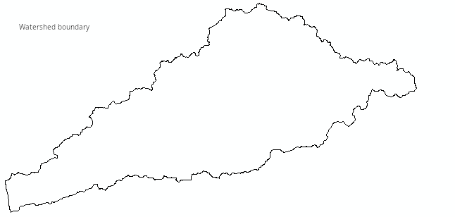
Download the worksheet here to a new folder called lab8 - if you are running Excel from your own computer make a subfolder in whatever folder you use for class files, or if you're running Excel through CougarAapps put it on your S: drive in a folder called lab8. Once it's downloaded open it in Excel. You'll see the first worksheet, labeled "Sampling_ndvi84", will allow you to simulate the process of sampling NDVI from within the public land in the "focused planning area" (FPA) of the San Dieguito River watershed. The San Dieguito River Park is attempting to assemble a park within the FPA that will allow a Park visitor to walk from the beach in Del Mar to the top of Volcan Mountain outside of Julian without leaving the Park. To be clear what the data are, the image below shows the now (very) familiar watershed boundary.
If you click on the map you'll see:
It is this NDVI image that we will be sampling from.
If you look at the Excel worksheet the map with NDVI within public land in the FPA is reproduced, overlaid with a set of 50 random points from which NDVI is measured. The x and y coordinates (in longitude and latitude, decimal degrees) are shown in columns B and C (A is hidden, and isn't needed), and column D has the NDVI for the points.
The sample of data we are using is being randomly selected from the full set of pixel values (in worksheet "NDVI_pts_do_not_edit"). Excel re-calculates whenever you make a change to a cell's contents, or if you hit the F9 key - find and hit F9 and you should see a new set of 50 points are selected every time, so that the columns of data change, and the points on the map change to show which pixels are being used.
Because this is a contrived example in which we actually have every pixel's NDVI measured, we can know that the average NDVI within public land in the FPA is equal to 0.45150197 - this value is calculated in cell F3, which is the mean NDVI from every pixel in the map (these values are in sheet NDVI_pts_do_not_edit). We will treat this as the population mean (also called the population parameter), and each sample mean we generate is an estimate of this value.
Estimating the population mean may sound like something new, but in reality any statistic that you calculate from a sample of data can be thought of as an estimate of what you would get if you had used a complete inventory for the population. This means that, for example, the sample mean is not only a summary statistic that describes the typical value of the sample of data, it is also an estimate of the population parameter. Estimating the population mean is just done by calculating the sample mean, which is what we will do now.
Help with Excel
But, before we proceed, bear in mind that these instructions assume you know how to use formulas and functions in Excel. I teach another class, Biol 365, that spends the entire semester teaching how to use Excel for various applications in the biological sciences, and the material from that class may be helpful to you if you are not familiar with use of Excel for doing calculations. If Excel is new to you, and you would like some tutorial material to learn the basics, have a look at my Biol 365 activity that teaches basic usage of Excel here, and the activity introducing cell formulas and functions here. Even if you feel comfortable with Excel, and have no trouble following the instructions below, you may learn something new from these pages, I recommend you take a look when you have a moment.
1. Calculate the mean for the current random sample.
In cell G7 enter the formula =average(d2:d51) - average() is an Excel spreadsheet function, which averages the cells entered as arguments within the parentheses. Using the arguments d2:d51 says "every cell between column D row 2 and column D row 51". Capitalization doesn't matter in Excel, so Average(D2:d51) works just as well (this will not be the same in R - enjoy it while you can!). When you hit ENTER you should see the mean of the 50 points. As soon as you hit ENTER a new set of 50 points is selected - this is intended, and we will make use of this behavior once you have your confidence interval calculated.
**Note that I have embedded comments in every cell requiring a calculation in this sheet - if you hold your mouse over the red triangle in the upper right corner of a cell a yellow box will pop up explaining what you need to enter in the cell, and what the calculation is doing**
2. Calculate the standard deviation for the current random sample, and enter the sample size.
What is the standard deviation? It is a measure of variability among the NDVI values in the sample. The formula for standard deviation (s) is:
The numerator is a measure of how far data values (xi) are from their group means (x̄) (the sum of squared differences from the group mean), and the denominator divides by a measure of how much information is available in the data for the estimate of the standard deviation. Degrees of freedom for a sample of data is sample size minus 1, because we need to estimate the mean to estimate the standard deviation (we will encounter degrees of freedom periodically throughout the rest of the semester, and although the formula is different depending on the procedure, in every case it will be based on a measure of how much data is being used with the number of estimates or constraints on the estimates there are deducting from the value).
But, you do not need to enter this formula, because Excel has a built-in function to calculate standard deviation, called stev(). Select cell G8 enter the formula =stdev(d2:d51) and hit ENTER - this will calculate the sample standard deviation.
Standard deviation is not a measure of how variable we expect random sample means drawn from the population would be, it is a measure of how much the individual NDVI measurements are. However, we will used this information about variability among data values to calculate a measure of the expected amount of variation among means of repeated samples (we'll get to that in step 3).
Now enter the sample size in G9 - this is 50, the number of points that are being randomly selected from the population.
3. Calculate the standard error.
Now we have a problem - we want to know how good this estimate of the mean is, but we don't seem to have the information we need. We would conclude that the estimate is good if we knew how close it was to the population mean, but aside from artificial examples like this one we don't know what the population mean is (if we knew that it would be pointless to estimate its value with a sample!).
Since we can't know how close an estimate is to the population mean, we can at least estimate how consistent the estimates would be - if we were to repeat our calculation with a new sample of 50 points we would not expect to get an identical sample mean, but the closer together the sample means are the more confidence we would have that the population mean can't be too far from the sample means. So, we can use the amount of variability among means of repeated samples drawn from the population as a measure of consistency in our sampling (or rather, as sampling variability, which is the opposite of consistency, but low variability would indicate consistent estimates).
If we had many, many repeated samples we could record their means and calculate the standard deviation between the sample means to measure sampling variation. We could do this with a computer simulation like the one we're working with, but usually we don't have the luxury of measuring a huge number of random samples of the same size to see how variable their means are. Fortunately for us, there is a simple relationship between the amount of variation among the measurements in a single sample of data and the amount of variation between sample means drawn from repeated samples, which is:

The standard error, symbolized by sx̄, estimates the amount of variability expected from repeated samples drawn from a population at a sample size of n. Although we only have a single sample, we can calculate the standard error from the standard deviation and the sample size, both of which are properties of a single sample of data.
Pause for a moment and consider how lucky this is - the information in a single sample of data is all we need to predict the amount of variation we can expect if we randomly sampled from the population many, many times. That this is true saves us a tremendous amount of sampling effort.
To calculate the standard error, select cell g13 and enter =g8/sqrt(g9) - this will take the standard deviation in G8 and divide it by the square root of the sample size in cell G9.
The standard error is a little hard to interpret by itself, and we usually use it as the basis for calculating a confidence interval. Confidence intervals give us a range of values that are plausible (i.e. reasonable, given the available information) values for the population mean. Over the next couple of steps we will use the standard error to calculate the confidence interval for our sample mean.
4. Calculate the t-value
The next problem to solve is that we have a standard error that indicates how much sampling variability to expect, but we don't yet know how many standard errors above or below the sample mean we would need to go to have a high chance of including the population mean.
Again, if we had the luxury of randomly sampling many, many could just see how far from the average of all the sample means we would have to go to capture, say, 95% of them. Since this isn't practical, we need a method that works even when we only have a single sample of data.
The solution we will employ here is to use a mathematical model of the sampling distribution. A sampling distribution is a curve that shows us how the estimates from repeated samples should be distributed. The mathematical model of a sampling distribution we will use is the t-distribution.
The graph below the map in your Excel worksheet illustrates how we will do this - the t-distribution is a probability distribution, meaning that the area beneath it is equal to 1. The t-distribution is centered on 0, which we take as the location of the estimated mean, and the x-axis values are in standard errors (we refer to these as t-values, but a t-value of 1 indicates 1 standard error away from the mean, and a t-value of 2 is 2 standard errors away from the mean, etc.). Since the total area beneath the curve is 1, the area under any subset of the curve will be between 0 and 1 (if no values under the curve are included the area is 0). This allows us to set a confidence level that we want to achieve - if we want to have a 95% chance that our confidence interval will include the population mean, we can shade 95% of the curve, symmetrically around the middle. The t-values below the middle (a negative t-value) and above the middle (a positive t-value) are the critical values between which 95% of the sample means will fall.
If we want to include 95% of the curve between our lower and upper critical values, we need to find the t-value below which 2.5% of sample means will fall on the negative end, and above which 2.5% of sample means will fall in the positive end - this will exclude a total of 5% of possible sample means in the "tails" of the curve, but between these t-values will fall 95% of the sample means. Since the t-distribution is symmetrical, the critical values will have the same magnitude (i.e. the same absolute value), but will have different signs. We can calculate the critical values in Excel, with the tinv() function.
Select cell g17 and enter the formula =tinv(0.05, g9 - 1) and hit ENTER - you should see the value 2.009575. This is actually the upper critical value, but since the t-distribution is symmetrical the lower critical value is just -2.009575, so we get both the upper and lower critical value with this one formula. The formula's first argument (0.05) is the amount of the curve we want to put in the tails (0.05 will put 0.025 in each), and g9 - 1 is the sample size in G9 minus 1, or 49. The t-distribution's shape is affected by the degrees of freedom, which for a confidence interval is n - 1.
Since t-values are numbers of standard errors, we now know that if we find the NDVI value that is 2.009575 standard errors below the mean, and the NDVI value that is 2.009575 standard errors above the mean, then the population mean will have a probability of 0.95 of falling between these points (or, if you prefer, there will be a 95% chance that the population mean falls between the lower limit and upper limit of this interval). Once we have calculated these lower and upper limits we will have our 95% confidence interval.
5. Calculate the uncertainty
The t-value has units of standard errors, but we need to translate 2.009575 standard errors into the same NDVI units as the mean. To convert our critical t-value into NDVI units we just need to multiply the t-value by the standard error.
The product of the standard error and the t-value is called the uncertainty of the estimate. To calculate it, select cell G18 and enter =g13*g17, and hit ENTER - this multiplies the t-value in G17 by the sample's standard error in G13.
6. Calculate the lower and upper limits of your confidence interval
Now that you have the uncertainty of the estimate you just need to subtract it from the sample mean to get the lower limit of the confidence interval, and add it to the sample mean to get the upper limit.
Select cell G20 and enter the formula =g7 - g18 and hit ENTER - this is the lower limit. Then, select G21 and enter the formula =g7 + g18 and hit ENTER - this is the upper limit.
All that step 5 and 6 have done is to first translate the critical t-value into NDVI units, and then add and subtract it to the mean to put the uncertainty around the mean - the graph below the t-distribution, with the title "The 95% CI for NDVI" shows the result - the red region is the 95% confidence interval, with the mean of your sample in the middle. The lower limit if the interval is 2.009575 standard errors below the mean, and the upper limit is 2.009575 standard errors above it. Usually we represent a confidence interval as a point with error bars around it, but this way of representing it shows how it is calculated, and why the upper and lower limits are placed where they are.
7. Does a 95% interval actually contain the population mean 95% of the time?
Now for the fun part... with the formulas all set up, every time you hit F9 to select a new sample the mean and confidence interval update as well. Because we have every pixel available to measure, the population mean NDVI is in cell F3, and we can test to see if it falls inside of the confidence interval for the current sample mean. To make this easier I have set the cell in F3 to turn red if the population mean is not inside the 95% confidence interval for the sample (if the population mean is either less than the lower limit or greater than the upper limit then it's outside of the interval). Since this is a 95% CI we would expect the population mean to be excluded 5% of the time, but is it? We can find out by sampling lots of random samples and counting how many of the intervals don't include the population mean.
I want you to hit F9 100 times, and count up how many times the population mean in F3 turns red. To help you keep track I have labels in cells F26 through F35 where you can record how many times the cell turns red for each 10 repetitions (don't want you to lose track after 72 and have to start over). So, hit F9 ten times and record how many times cell F3 turns red, then repeat this process ten times.
When you're done, in cell G37 enter the formula =sum(g26:g35), and you should have roughly 5 intervals that didn't contain the population mean (give or take a few, this is random sampling).
Answer the three questions in the Sampling_ndvi84 tab, and you're done with estimation - you can save the file and move on to the inferential statistics review.
Inferential statistics is about using the information in a sample of data to evaluate hypotheses about populations. You will learn about alternative approaches later, but the methods of inferential statistics you learned in your introductory statistics classes were probably limited to testing hypotheses, to establish whether an apparent pattern in the data is likely to actually be due to random chance (i.e. the null hypothesis), or to an actual relationship between variables (i.e. the alternative hypothesis).
We will review two, related inferential statistical methods - linear regression and analysis of variance (ANOVA). In both cases we seek to explain variation in one variable (called the response variable) using another variable (called the predictor variable). The only difference is that in ANOVA the predictor variable is categorical, made up of discrete levels, whereas with linear regression the predictor is numeric. In both cases the response variable is numeric. The differences between the methods is superficial, and both are actually examples of a general linear model - if you want to learn more, take Biol 531!
For the review exercise I sampled NDVI from the spring for three years, 1984, 1998 and 2011, using two different sampling designs:
Since the three years can be treated either as a categorical grouping variable or a numerical predictor, we can analyze the data using either ANOVA or regression (although you will see only one of these two is really appropriate for these data).
We will be using a program called R to do our statistical analysis for this exercise. R is actually an object-oriented programming language, which can be used interactively to analyze data. It is extremely powerful, but not very user friendly (I prefer to think of it as user hostile). If you were to download, install, and run R by itself you would see a program that looks like this (on Windows - it would be similar on a Mac, and even more rudimentary in Linux). The "R Console" is where commands are issued, and the graphical user interface (or GUI) that is distributed is very rudimentary - there are no menus for running statistical analyses or making graphs like you get with MINITAB, and all of the menu selections and buttons are for opening and saving R's "workspaces", printing output, or managing add-on packages. There are also some fairly simple things (like having more than one graph displayed on the screen at the same time) that are difficult to do.
There are graphical user interfaces that have been developed that use R for all of their calculations, but provide a menu-based interface, much like MINITAB - one that I think is particularly interesting, and considered using for class is called Jamovi, which you can get from https://www.jamovi.org/ if you are interested. Jamovi has a fairly good selection of analysis types built in, with more that can be added through extension packages. But, we don't currently have it available through CougarApps, and I wanted to stick with something that I could be certain everyone would be able to run one way or the other, so we won't be using it in here.
In the long run, to get the most out of R it's good to learn to use the command-line interface, but it's helpful to have some guidance with basic things. Between the extremes of using a full-blown graphical interface vs. running everything directly in R, there are are "integrated development environments" (or IDEs) designed to help us use R more efficiently and easily. There are several IDEs available, but in my opinion the best is R Studio. R Studio does not provide a graphical interface to R's statistical analysis, but it is a graphical interface to such useful things as accessing help files, browsing for and importing data files, managing graphs, and editing R commands. It also helps organize your work, and provides a very nice system for documenting your analysis. It is the tool I use in my own work, and it is well worth the effort to learn.
The best way to use R and R Studio is to install them on your own computer. It isn't hard to get them installed, and both run on Windows, Mac OS, or Linux. If you can't install them on your own computer for some reason, it is possible to run both through Cougar Apps, but I recommend against relying on this - it will be more likely to crash, and there is an annoying bug that only crops up when you run R Studio via Cougar Apps that will make it harder for you to produce the Word documents at the end when you complete your analysis. If you want to run R Studio through CougarApps the instructions should still work, and you can skip over the installation steps..
To get up and running, you will need to first install the most recent version of R, then install the most recent version of R Studio.
First, install R:
Next, you will want to install R Studio:
You should now be able to start R Studio (you will see that R is installed and can be run on its own, but there's no need - you will always use R via R Studio in this class).
Now we can launch R Studio for the first time. Note that some of R's functionality is provided by external packages, called libraries in R, that are not part of the base package. If the first time you launch R Studio you are asked if you want to install some additional libraries it says it needs, say yes.
When you run R Studio, you will see a window that looks like this:
If you move your mouse over the picture above you'll see popups that indicate the location of the:
You will learn what a few of these are for in this exercise.
A quick note about the Help files.. you may not find them all that helpful. One of the downsides of using an open source package is that the help files are not always very beginner friendly. This is because the help files are written by the software developers, who are expert statisticians as well as experts in R, and they assume you are also an expert statistician who knows R and only need to know how to make the particular command in question work. The explanations will often be too sophisticated to be helpful right now. Consider me, and the materials I provide you, to be your Help file for now, and don't hesitate to ask if you have trouble.
One of the best features of R Studio is that it helps organize your work, using projects. Projects are a folder that contains all of the files needed for the analysis task you are completing, including the data sets and commands you used. You will want to get into the habit of starting each assignment with a new project, so that you don't end up with a confusing mess of files from different projects all mixed into one place.
To make a new R Studio project, do the following:
Once you're done you'll see that the Environment tab is blank, except for a gray "Environment is empty" label, and the "Files" tab shows a file that is named for the folder you used, with a .Rproj extension - this is the new project file that R Studio just created. Project files are like the map files that ArcMap creates - they don't contain data sets or a history of the commands you've used, those will be in files called .RData and .Rhistory respectively, but the project file does record things like the window states, so that when you come back to the project later it will open up all the windows you were using so that you can pick up where you left off. Two files, called .RData and .Rhistory, will be created the first time you save, but you won't have them in your Files tab yet. These are important, don't delete them, but you won't be interacting with them directly - R Studio will take care of saving the workspace (.RData) and command history (.Rhistory) each time you save the project. Again, like ArcMap, a project in R Studio is made up of multiple files that all have to be in the right place (preferably, in the project folder) for things to work right.
Assuming you did use the folder with the Excel file from the estimation step, you should also see stat_review.xlsx in the Files tab.
The thin status bar just above the "Name" label shows that you are looking at the contents of the new folder you just created. This is your working directory, which R will use for output files, and where it will look for any input files unless you tell it otherwise. By default, when you make a new project R sets the working directory to the project folder for you (it's possible to use something else, but if you are using projects to organize your work it's best to use the project folder as your working directory).
A good way to start learning R is to enter some simple commands in the Console. R commands are entered to the right of the bottom-most prompt, which is the blue greater-than symbol, >. A simple R command is:
5+5
I'll use a font and color for commands that look like the Console to help you identify the commands you're meant to enter from these instructions - enter this command next to the prompt and hit ENTER, and you will see just below your command the output:
[1] 10
The 1 in square brackets is an index number - it just says that 10 is the first element of the output, and the value 10 is indeed 5+5.
R is object-oriented, meaning that it is designed to work in a way that is similar to objects in the real world work. What I mean by this is easier to understand through a simple example.
First, let's make a vector of numbers - a vector is just a set of elements that can be indexed with a single number. You make a vector in R with the c() function:
c(2, 4, 6, 8, 10)
If you hit Enter you will see output:
[1] 2 4 6 8 10
You still only see [1] as the index, because R only reports the index number at the beginning of the row of output, to keep the output compact. But, this is a vector with five elements - the first element has a value of 2, the second has a value of 4, and so on.
The output of our command was reported to the console, but it wasn't saved into an object. To assign the output of this c() command to an object, use the up-arrow key on your keyboard (↑) to recall the command, and edit it to read:
numbers <- c(2, 4, 6, 8, 10)
If you hit ENTER you won't see any output in the console this time, but you will now have an object in your Environment tab called numbers, and the contents of the object are displayed to the right of its name. The <- (less than followed by a dash) together make a left-pointing arrow, which is called the assignment operator in R - it tells R to take the vector we're creating on the right side of the arrow and assign it to the object with the name numbers on the left. You can use a right-pointing arrow instead; we could have used:
c(2, 4, 6, 8, 10) -> numbers
to accomplish the same thing.
The Environment tab gives you a brief preview of what the numbers object contains, and since numbers is a short vector of only five elements you can see all of it. Another way to see the contents of an object is to display it in the console by entering its name - if you type:
numbers
and hit ENTER the five numbers this object contains are displayed in the console.
You can use objects in other commands by typing their names - for example, if you want to add 10 to each number you would use:
10 + numbers
to get:
[1] 12 14 16 18 20
You can see that this command added the number we specified (10) to each element in the numbers vector. Since we didn't assign this output to an object it is reported to the Console, but it isn't saved anywhere.
Most of the time we will be using R functions rather than typing in the formulas for doing calculations. Functions are commands that have a name followed by parentheses (with no space between the name and the left parenthesis), with arguments within the parentheses that provide the function with instructions about how to work, or with data to work on. We have already used one function, the c() function, which creates a vector out of the arguments within the parentheses. For our second function, we can use summary() on our numbers object to summarize its contents:
summary(numbers)
which gives us this output:
Min. 1st Qu. Median Mean 3rd Qu. Max.
2 4
6 6 8
10
You may recognize this from your introductory statistics class as the five number summary (minimum, first quartile, median, third quartile, maximum), along with the mean of the data - this is a useful way to summarize numeric data, and you can use it to see if the data are skewed (if the data are skewed the median and mean will not be the same, and the spacing between the median and the quartiles or the maximum and minimum will not be equal).
One of the defining characteristics of an object-oriented language like R is that the same command applied to different kinds of objects gives you different results, just like real objects in the real world. For example, if I asked you to summarize a set of data you would give me a set of summary statistics, but if I asked you to summarize a movie you would tell me about the plot - thus, even though the command you received was the same, the method you used would be selected to match what you were summarizing. Likewise, in R the same summary() function will give different results if we apply it to a vector of text, instead of a vector of numbers. To demonstrate this, make a vector of words called text, like so:
text <- c("blue","green","red","yellow","orange")
You will see that you now have a second object in your Environment called text, but its type is shown as "chr" (for "character") instead of "num" (for "numeric"), and its elements are the five colors you entered. The words are all enclosed in quotes (either single or double quotes would have worked, as long as they match) to indicate that these are text labels rather than names of objects.
What happens if you type a word without quotes? R assumes a word without quotes is supposed to be an object name, and gives you an error message when it can't find that object in your Environment. For example, if you had entered:
c(blue, green, red, yellow, orange)
you would get the message:
Error: object 'blue' not found
Because the word blue isn't quoted, R assumed it to be an object name, looked for the object called blue in your environment, and gave you an error when it couldn't find it (this was a fatal error, meaning that the function couldn't proceed to the next argument after encountering it, so it hasn't looked for green, red, yellow, or orange yet, but they too would have caused the same problem).
Get to know this error, by the way, you'll be seeing it a lot... the other very common way to get it is to misspell an object name, or to use the wrong case (lowercase when you should have used uppercase, or the reverse) in your command. Embrace it, it will be your companion (I've been using R for 20 years, and I still get plenty of them) - when you see it, start looking for typos.
R objects have methods, which are instructions for what to do when a command is applied to them. If you use the same summary() command on the text object that we used on the numbers object:
summary(text)
you will get output:
Length Class Mode
5 character character
This output is different, because the summary method for a vector of text is different than for a vector of numbers. It wouldn't make sense to try to calculate the mean of five words, so R doesn't do that - instead, it tells us this vector has five elements in it (length of 5), and has a Class and Mode of character (don't worry about the difference between Class and Mode, it's not important to us at this point, but both are indicating this vector is a bunch of character data rather than numbers). This means that the same function can be used on objects of different type to get output that is appropriate for that object type.
A quick note about object types - if we had entered:
c("2","4","6","8","10")
then the output would have shown us the numbers with quotes:
[1] "2" "4" "6" "8" "10"
indicating that they are being treated as text labels, rather than as numbers. If we summarized this vector of numbers as text, we would get:
summary(c("2","4","6","8","10"))
Length Class Mode
5 character characterSo, entering the numbers quoted makes R treat them like text, and changes how they are summarized.
Also, notice that we didn't need to make an object of the quoted numbers before summarizing them - we could use the c() command as an argument for the summary() command instead. When R sees this, it works on the functions from the inside out - it evaluates the c() function by making a vector of quoted numbers, then passes the text vector created by c() to the summary() function, which summarizes the output.
Nesting commands is something we will do periodically, but I think it makes code more difficult to understand, and is less beginner-friendly, so we will use it sparingly (in this case, we could have assigned text-mode numbers to an object and then applied the summary command to that object, which makes it clearer what each part of the command is doing). If you do use nested functions, watch those parentheses - you need a close parentheses for every open one, and if you forget to close a parenthesis things get very confusing (R thinks you're making a multi-line command when you hit ENTER and changes the prompt to a + and awaits the rest of the command).
You can refer to the elements of an object by index number using square brackets at the end of the object name - for example, to see the fourth word stored in text you would use:
text[4]
will show you the fourth element in the text object, which is the word "yellow".
We have been working in the Console so far, but that's not how we will be completing most of our work in here. Time to move on to the assignment for today.
We will be using a file format called R Markdown any time we use R in this class. R Markdown is a formatting language that allows us to use symbols to indicate how an output file created from the inputs we write will look. Markdown is a actually a pun, in that it is meant to be a simplified version of a markup language (such as HTML, short for hypertext markup language, which is used to format web pages like this one). But, in addition to formatting instructions, R's markdown format allows us to mix R commands into our document, which are executed when an output file is created.
There are several major advantages to using R Markdown that make it useful not only for teaching and learning R, but as the platform for your own data analysis outside of class:
R Studio's support for R Markdown is excellent, in that it makes the code chunks in a markdown file executable - you'll be able to enter code within the Rmd file, run it, and get output from it within R Studio, just like you would if you were working in the Console.
I will be providing you with templates of R markdown documents for each exercise - this week's file is here. **I accidentally posted a worked copy of the file, with all the commands already in the code chunks... if you want something a little more challenging, try this file, which has most of the code chunks blank.** The file is a simple text file, so when you click on the link your browser helpfully opens it in a new tab, because that's what browsers do with simple text files. But you don't want that, you want to download it, and you want to preserve the .Rmd file extension so that R Commander can use it properly.
To download the file instead of opening it, right-click on the link (if you have a two button mouse) or CTRL+click the link (if you have a one-button mouse), and select "Save link as..." (or whatever version of this command your web browser provides). You will then be given a download window that lets you select the location to download the file - save it into your project directory (you'll see it in the Files tab of your project).
Markdown files will have the filename extension .Rmd, so I'll refer to them as rmd files for short.
Once the lab8_stats_review.Rmd file is in your project directory, click on its name in the "Files" tab to open it, and you should get a new tab open that shows you the contents of the file - it should look similar to this image below - this is actually from a different file that has several of the relevant pieces close together, which is better for illustrating the structure of the file (you can hover over parts of the file to get popup notes about what each section is):
You will find the following:
To complete this part of the assignment follow the instructions in the Rmd file.
When you are done you will "knit" your Rmd file to create a Word document, and upload that along with the Excel file with your confidence interval review to the class web site.
We are just scratching the surface with R in this class. There are several good, free tutorials on R that you can use if you want more than you get in here.
A good place to look for them is the CRAN web site - go to http://cran.r-project.org, and find the "Documentation" links on the left side of the page. The "Manuals" are meant as complete references, but are not written as tutorials. The "Contributed" documentation section gives several good introductory documents that you can check out. Some particularly newbie friendly ones are "R for Beginners", and "Kickstarting R". Another good, fairly comprehensive document that uses biological examples is "Statistics using biological examples".
The graphical interface we're using, R Commander, is a "contributed package" that isn't a standard part of R. Consequently, it will most likely not appear in the tutorials linked above. If you want to learn more about how to use it, you can try "Getting Started with the R Commander" (written by the guy who programmed R Commander), or possibly "R Commander: An Introduction" (written by some other person).
If you like actual dead-tree books better, there is now an "R for Dummies" book (if your pride allows it). A couple other good options include "Introductory Statistics With R", and "A Beginner's Guide to R", which cover similar ground as the Dummies book without requiring you to eat humble pie. Finally, "R in a Nutshell" is a good reference, but with less emphasis on teaching.