Introduction

You may have heard the myth that the Swiss would tie barrels of brandy
to the necks of St. Bernard rescue dogs to warm up cold skiers in the
Alps (this gif is from a Disney cartoon that depicts a St. Bernard
giving a very cold Pluto a shot from his barrel. Binge drinking is not
usually depicted in children's cartoons anymore - it was 1936, times
have changed). The basis of this myth is the belief that drinking
alcohol increases body temperature because people experience the
sensation of warmth after drinking it. But, this subjective feeling of
warmth may or may not reflect an actual increase in core body
temperature.
How would we know if drinking brandy actually changes body temperature?
As data-driven scientists, we should try to answer this question by
devising an experiment to test whether drinking brandy changes core body
temperature (and, no, this is not what we'll be doing in class this
week, sorry to disappoint you).
As you know from our work on experimental design, to test the effect of
brandy on body temperature we need to apply a treatment (brandy
drinking) and measure a response (body temperature). One possible
experiment that would test the hypothesis that drinking brandy affects
core body temperature would be:
- Administer a shot of brandy (1.5 fl. oz.) to a randomly selected
group of people (our experimental subjects).
- Measure each person's core body temperature.
- Compare the mean of the measured body temperatures to 98.6° (average
normal core body temperature for humans - the body temperature we
would expect if brandy has no effect on body temperature). We would
draw a conclusion based on these decision rules:
- If mean body temperature is higher than 98.6°, conclude that
drinking brandy increases core temperature.
- If mean body temperature is equal to 98.6° conclude that drinking
brandy doesn't affect core temperature.
- If mean body temperature is less than 98.6° conclude that drinking
brandy decreases core temperature.
Brandy experiment: results
x̄ = 98.7°
s = 0.3
n = 20
If we conducted the experiment and got the results in the box on the
right, the decision rules tell us that since the sample mean body
temperature of x̄ = 98.7° is above 98.6° we should conclude that
brandy increases body temperature.
That's what the data says, and you can't argue with the data. Right?
Random sampling strikes again
Unfortunately, it isn't so simple.
The problem is, the decision rules are not accounting for random
sampling. According to the decision rules we can only conclude that
drinking brandy doesn't affect core temperature if the mean for our data
is exactly equal to 98.6°, and any differences, no matter how
small, would cause us to conclude that brandy either increases or
decreases body temperature.
This is a problem because the random samples we work with will produce
some random variation in sample means. So, even if the population mean,
μ, is exactly equal to 98.6°, the mean of a sample selected from that
population, x̄, probably won't be. These differences would cause us to
conclude that there is an effect of brandy on body temperature when
there is not if we used decision rules that didn't account for random
sampling.
The simulation to the right illustrates the problem - the data points
represent a sample of 20 body temperatures selected from a population
with a body temperature of μ = 98.6°, and the mean of the sample is
reported below the graph. If you click the "Select a random sample"
button a new sample of 20 is selected from the same population, which
gives you a new sample mean. As you click repeatedly, note that the
sample mean is rarely equal to 98.6°. Because of this random sampling
variation, if we conclude that any mean other than exactly
98.6° indicates that brandy has an effect on body temperature then we
will mistakenly conclude that brandy has an effect most of the time.
If you keep hitting "Select a random sample" you'll see that even
though the mean is changing randomly, it isn't completely unpredictable.
Means exactly equal to 98.6° don't happen very often, but means only
rarely go as low as 98.5° or higher than 98.7°. This suggests a solution
to our problem - even though a mean that is exactly equal to 98.6° isn't
likely, we can change our decision rules to reflect the fact that small
differences can happen by chance. If we can characterize the range of
variation in sample means that random sampling usually produces then we
can treat any observed difference that's within this range as probably
being due to random chance, but treat sample means that fall outside of
this usual range as probably being due to an actual effect of brandy on
body temperature.
The question is, then, how different from 98.6° would our sample mean
have to be to conclude that brandy has an actual effect on core
temperature?
To
answer that question we need inferential statistics,
which are methods that allow us to draw conclusions about a population
based on a sample of data. This week we will learn how to do a
type of null hypothesis significance test (NHST),
called a one-sample t-test, to determine if our sample
mean of x̄ = 98.7° is different enough from 98.6° to conclude that
drinking brandy increases body temperature.
Inferences are based on hypotheses
Before we learn about the one-sample t-test we will use in particular,
we need to spend a little time on NHST's in general.
In the sciences, we base our conclusions on tests of hypotheses.
In the sciences, a hypothesis is simply a possible explanation for some
phenomenon. In inferential statistics we will call these sorts of
statements of the way we think a system is working scientific
hypotheses, although sometimes we will simply refer to the
scientific hypothesis as the question we are trying to answer. For the
current example, the scientific hypothesis is that brandy increases body
temperature. The experiment we designed to test this question has us
measuring body temperature, and we came up with some decision rules that
tell us how to interpret the three possible outcomes of our experiment
(i.e. an increase in temperature, no change, or a decrease in
temperature). We use the scientific hypotheses to guide us in developing
statistical hypotheses, and we revisit the scientific hypothesis after
our statistical analysis is complete to draw a conclusion about whether
the experiment supports our scientific hypothesis. This final decision
will be based on our decision rules, modified to account for the effects
of random sampling.
Statistical
hypotheses are about how randomness affects our data. To decide if the
data gives us enough evidence to conclude that drinking brandy changes
body temperature we will test a null hypothesis. Null
hypotheses are always hypotheses of no difference, or randomness. We can
express a null hypothesis about our test of the effect of brandy on core
body temperature as:
Null hypothesis: at a population level, average body temperature
(μ) for people drinking brandy is 98.6°.
In other words, since we know that body temperature for people who
aren't drinking brandy is 98.6°, body temperature should still be at the
normal human body temperature of 98.6° if brandy has no effect. If the
null hypothesis is true, any difference between our experiment's sample
mean and this hypothetical population value is just due to random
sampling variation.
We test the null hypothesis, but there is another possibility - brandy
may have an actual effect on body temperature. We do not know what the
body temperature of people who drink brandy should be, but if brandy
affects core temperature it definitely shouldn't be 98.6° anymore. We
can thus express this alternative hypothesis as:
Alternative hypothesis: at a population level, average body
temperature (μ) is not equal to 98.6° for people drinking brandy.
You can see that a null hypotheses is very specific - it specifies a
hypothetical value of the population mean exactly. In contrast,
alternative hypotheses are not specific at all, they just say "whatever
the population mean might be, it is not equal to the null value".
So far this doesn't actually look any different from the decision rules
that we set up before. There is a very important difference, though - the
null hypothesis is about the population mean, not about the sample
mean. We will use the value of the population mean of 98.6°
as the center of a sampling distribution, and will ask if the sample
mean of 98.7° that we observed is likely to occur by chance, or unlikely
to occur by chance when the null hypothesis is true and brandy has no
effect on body temperature. This will account for random sampling, and
will allow us to draw a conclusion about our scientific question in a
way that properly acknowledges the way that randomness affects our data.
The general procedure that all null hypothesis significance tests
follow is:
Formal null hypothesis
significance testing
- State the null hypothesis - in terms of hypothetical values of a
population parameter.
- Calculate a test statistic from the data that
measures how far the data are from the value specified in the null
hypothesis.
- Compare the test statistic to a sampling distribution to obtain a
probability of the test statistic, if the null hypothesis is true
(the p-value).
- Compare the p-value to a predetermined level, called the α-level
- If p is less than α reject the null in favor of the alternative
hypothesis.
- If p is greater than α retain the null hypothesis.
- Draw a scientific conclusion, based on the result of testing the
null hypothesis.
The one-sample t-test
The above set of steps are common to all NHST's, but the details are
different depending on the data type and experimental design used. In
this body temperature experiment example, we have:
- One sample of data: 20 people
- A continuous numeric variable: body temperature
- A known, hypothetical value we will compare out sample of data to:
98.6°
The appropriate null hypothesis significance testing procedure to
compare a single sample mean to a specified hypothetical population mean
is called a one-sample t-test.
The steps in the procedure are as follows:
1. State the null (and the alternative)
The null hypothesis will always be the hypothesis of no effect or
randomness, and it will be expressed in terms of a population parameter.
If there is no effect of brandy drinking we expect the population mean
to equal 98.6°.
To make the null hypothesis as precise and clear as possible we can
express it in symbolic form. The symbol for "null hypothesis" is Ho, or
"h-naught", with the o representing a subscripted zero.
We can write the null hypothesis symbolically as:
Ho: μ = 98.6°
or, equivalently, as:
Ho: μ - 98.6° = 0
This makes it absolutely clear that our null hypothesis is that the
mean of the population our data was selected from is 98.6°.
Once the null hypothesis is stated, the alternative
hypothesis is just that the null hypothesis is false.
Symbolically the alternative hypothesis is:
HA: μ ≠ 98.6°
This statement makes it absolutely clear that if we decide that the
null is not true then all our null hypothesis test will tell us is that
the population mean is something other than the null value of 98.6°.
2. Calculate a test statistic
The test statistic tells us how different our sample
mean is from the null hypothetical value. Mathematically, "difference"
implies subtraction, so we could find the difference by subtracting our
hypothetical population mean of 98.6° from the sample mean of 98.7°,
which gives us 98.7° - 98.6° = 0.1°.
If you recall from our work on confidence intervals, we can use the
t-distribution as a mathematical model of randomly sampling means with a
given sample size from a population. The advantage of using the
t-distribution is that it will allow us to calculate a probability of
obtaining a difference of 0.1° from a population with a mean
of 98.6° based on the data in just a single sample. But, the units
on the x-axis of a t-distribution are standard errors, not degrees
Fahrenheit. To use the t-distribution we need to convert the units for
our difference into standard errors.
To do this unit conversion we first need to know the standard error for
the data set. The standard error for a single sample of data is just the
standard deviation divided by the square root of the sample size. Our
sample of 20 people had a standard deviation of 0.3, which means that
the standard error would be:

The units on a standard error are the data units, so there are 0.067°
in one standard error for this sample of data.
Now to get our observed t-value test statistic we just need to know how
many standard errors 0.1° is. This is just a simple unit conversion,
just like converting 120 inches into feet - to make this conversion we
would divide 120 inches by the number of inches per foot to get 120/12 =
10 feet. Dividing our observed difference of 0.1 by the number of
degrees in a standard error gives us:

This tells us that 98.7° is 1.49 standard errors above 98.6° (to be
clear, it's 1.49 standard errors away from 98.6°, and since
the value is positive it's above 98.6°). This observed t-value
is now in the correct units to compare to a t-distribution to obtain a
probability for our experimental result.
3. Compare the test statistic to a sampling distribution to obtain a
p-value
To reach our conclusion about the null hypothesis we need to calculate
a probability, called a p-value. The p-value is the
probability of a very specific thing:
The p-value is the probability of randomly sampling from a
population with a mean equal to the null value (μ = 98.6°) and
obtaining a sample mean that is at least as different from the null
value as the observed sample mean (x̄ - μ
= 0.1°).
We will use the t-distribution to obtain the p-value for our observed
t-value. Remember from the confidence interval exercise that the
t-distribution is a good mathematical model of a sampling distribution
for means, and its shape depends on degrees of freedom. For a one-sample
t-test degrees of freedom equals the sample size minus 1, which this
example is 20-1 = 19.

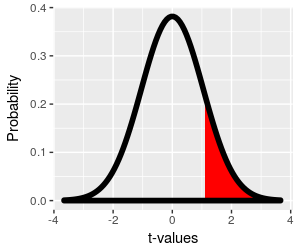
The t-distribution with 19 degrees of freedom is shown in the
graph to the left.
The probability of getting a sample mean at least t = 1.49
standard errors above 98.6° by chance is the red shaded area
from 1.49 to infinity, which is equal to:
p = 0.076
Finding the probability for an observed t-value is best left to
the computer - we will use MINITAB to calculate all of our
p-values for us.
This p-value is called a one-tailed p-value,
because we are only using one tail of the t-distribution to
obtain it. We suspect that drinking brandy increases body
temperature because it feels like it does, so we may only be
interested in the chances that random sampling would produce
sample means that are higher than 98.6° - if that's the case
then using a one-tailed p-value is appropriate.
|

However, it's possible that the sensation of warming when we
drink brandy is misleading, and that body temperature actually
decreases even though we feel warmer. This sort of unexpected
result can happen, and we may want to leave open the possibility
of the unexpected occurring when we do our work. When we're
doing our null hypothesis test we're considering the possibility
that our experimental result is only different from 98.6° due to
random sampling, and from that perspective the direction of the
observed difference isn't important - if it's a randomly
generated difference it could just as easily have gone the other
way. We account for this possibility by looking at random
differences that are just as big as we observed (0.1°, or 1.49
standard errors), but in the opposite direction.
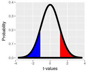
We account for the possibility of unexpected results by using a
two-tailed p-value. To include differences as
big as we observed in either the positive or negative direction,
we would want to include the blue region, which starts at t =
-1.49 and extends to negative infinity, as well as the red
region, to calculate our p-value.
Since the t-distribution is symmetrical, the area in the blue
region is also 0.076, and the two-tailed p-value that uses both
the red and blue regions is p = 0.152.
|
The way to indicate if your p-value is based on one tail or two is in
the way you represent the alternative hypothesis. If you are only using
the upper tail for the p-value you are only testing for a warming
effect, and your alternative hypothesis should be:
HA: μ > 98.6°
If you are testing for an effect of brandy on body temperature, and are
interested in finding either an increase or decrease in body
temperature, then your alternative hypothesis should be:
HA: μ ≠ 98.6°
We're using the HA: μ ≠ 98.6° alternative, so we would be
able to detect either an increase or a decrease in body temperature.
Obviously, if you wait to see which direction the difference was and
then tested for that direction of difference you would not be conducting
a fair, unbiased test. You should always decide whether you're testing
for just one direction of change or either direction before
looking at your results.
Given this explanation, what should the alternative hypothesis be if
you were only interested in testing for a reduction in body temperature
from drinking brandy? Click
here to see if you're right.
If you were only testing
for a reduction in body temperature the alternative hypothesis would
be HA: μ < 98.6°.
As a general rule, I would recommend using two-tailed tests unless you
have a really good reason to use one-tailed tests. It's better to leave
open the possibility of an unexpected result. For the brandy experiment,
we may think that brandy increases body temperature because drinking it
makes you feel warm. But, it is possible that drinking brandy produces
that feeling of warmth by moving some of the heat from the core of your
body to the surface, which could decrease core body temperature in spite
making your skin feel warm. Either possibility would be interesting, and
we should use the two-tailed p-value for our test so that either result
is detectable.
4. Compare p to α - reject the null hypothesis if p < α, and retain
the null hypothesis if p ≥ α
We now have a p-value of 0.152. You can think of this as telling you
that if drinking brandy has no effect on core body temperature a
difference of 0.1° away from 98.6° would happen 15.2% of the time.
This seems like a pretty high probability of the result being due to
random chance, and thus not due to a real effect of brandy, but how do
we know that p = 0.152 is big enough to conclude that brandy has no
effect?
Unfortunately, the answer is that we can't know for sure, because the
only probabilities that indicate certainty are p = 0 (impossible) or p =
1 (definite). Any time we draw a conclusion based on a probability other
than 0 or 1 leaves open the possibility that we are wrong. We can't
achieve absolute certainty about whether our result is due to random
chance or not, but we can decide in advance of conducting the test how
low the p-value has to be before we conclude that brandy has an effect.
We call this threshold value against which we compare our p-value the alpha
level, or simply α.
It's up to the data analyst to set alpha, but even though any value could
be used it's traditional to set alpha to 0.05. We draw our conclusion
about the null hypothesis using the decision rule:
- If p is less than 0.05, reject the null in favor of the alternative
hypothesis.
- If p is greater than 0.05, retain the null.
Our p-value is p = 0.152, greater than 0.05, so we retain the null.
COMMIT THIS DECISION RULE TO MEMORY! This is a very simple rule, but it
only works if you remember it!
We already met this decision rule when we were testing normality of
data, but in a different form. We "failed" the normality test when p was
less than 0.05, and "passed" it when p was greater than 0.05. The AD
test of normality is in fact a null hypothesis test, with a null
hypothesis that your data are normally distributed. If p is greater than
0.05 you retain this null (and "pass" the test), whereas if p is less
than 0.05 you reject this null (and "fail" the test).
By the way, statisticians often prefer to use fail to reject
or retain when they talk about the null, rather than accept,
because doing so acknowledges that this hypothetical value may still be
incorrect, but that our data provides too little evidence against 98.6°
as the value of μ to reject it.
5. Draw a scientific conclusion
We retained the null hypothesis that body temperature is equal to 98.6°
at the population level. Given this, scientifically speaking we do not
have sufficient evidence from our sample mean of 98.7° to conclude that
people who drink brandy have a body temperature that is different from
98.6° on average.
If you retain the null hypothesis, you can say your result is not
statistically significant. If p had been less than 0.05 we
would have rejected the null, and we would have been able to call the
difference statistically significant. This phrase can cause mischief,
because "significant" and "important" are synonyms in everyday usage,
but not in statistics. If you say your results are significant, all you
are saying is that your results are unlikely to be due just to random
chance, but that isn't the same thing as saying they are biologically
important. Biological importance can only be judged based on what you
know about the system - if an increase of 0.1 had in fact been
statistically significant, would that much increase be enough to use
brandy drinking as a way to stay warm? Would such a small increase in
body temperature be worth the mental impairment in a survival situation?
Such questions aren't addressed by the null hypothesis test - all you
learn from the null hypothesis test is whether you're justified in
considering your results to indicate a real effect of the treatment you
used, or more likely to be due to random chance.
So, now that we understand null hypothesis significance testing, let's
return to the logical setup for our experiment. The only change we need
to make is in the decision rules, and the changes are in italics:
- Administer a shot of brandy (1.5 fl. oz.) to each experimental
subject
- Measure each person's core body temperature (with an ear
thermometer)
- Compare the average body temperature to 98.6°.
- If body temperature is statistically significantly
greater than 98.6°, conclude that drinking brandy increases core
temperature.
- If body temperature is not statistically significantly
different from 98.6° conclude that drinking brandy doesn't
affect core temperature.
- If body temperature is statistically significantly less
than 98.6° conclude that drinking brandy decreases core temperature.
Now when we assess our results we don't base the decision on whether
the sample mean is equal to 98.6°, we base the conclusion
on whether the sample mean is significantly different from
98.6°. This change properly accounts for the way that randomness affects
our data, and prevents us from interpreting small, random fluctuations
as though they indicate real biological effects.
What does it mean to accept the alternative?
When you get a statistically significant result, you reject the null
hypothesis and accept the alternative hypothesis. The alternative
hypothesis is HA: μ ≠ 98.6°, which just states that the null
is wrong. The alternative hypothesis is not
that the population mean is equal to the sample mean; that is,
definitely not HA: μ = x̄ = 98.7°.
It's important to realize this, because researchers often act as though
rejecting the null is evidence that the population mean is equal to the
sample mean. This is actually a perfectly sensible thing to do, because
when the null is rejected the best estimate we have about the actual
value of the population mean is the estimate we get from our sample
mean. But bear in mind that the reason for treating 98.7° as the value
for μ is because it's the value estimated by x̄. Whether it's at all a
good estimate should be evaluated by calculating a confidence interval -
a narrow interval around 98.7° would indicate that you have good reason
to treat it as the correct value for μ. Understand, though, that the
alternative hypothesis doesn't give evidence for any particular value of
μ, only against a very specific value of μ, and is therefore by itself
not good evidence that μ is equal to the sample mean.
Formal null hypothesis testing - the critical t-value approach
So far, you've learned to compare a p-value to an alpha level to
determine whether to reject or retain the null. An alternative approach
that you will also see frequently in the scientific literature is to
compare the observed t-value to a critical t-value.

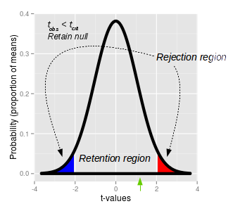
This graph of a t-distribution illustrates the approach. Once
we pick an alpha level of 0.05, we can put 1/2 of it in the
upper tail and 1/2 in the lower tail, which defines the upper
(red) and lower (blue) rejection regions. The
t-values that define the ends of the shaded regions are the critical
t-values. The critical t-value for our experiment,
with 19 degrees of freedom is tcrit = ±2.1. If an
observed t-value falls into either of these rejection regions
the probability of observing a t-value of that size is less than
0.05, and we would reject the null.
Between the critical t-values of -2.1 and 2.1 is the retention
region. Any t-value that falls within the retention
region has a probability of occurring that is greater than 0.05,
and would cause us to retain the null.
Our observed t-value of 1.49 (shown by the green arrow below
the x-axis) falls inside of the retention region - thus, we
retain the null, and conclude there our sample mean of 98.7 is
not significantly different from 98.6.
If you click on the picture you'll see that it changes between
a p-value approach and a critical t-value approach so you can
see how the two methods are related.
|
|
α(2): t0.20 |
t0.10 |
t0.05 |
| df |
α(1): t0.10 |
t0.05 |
t0.025 |
| 1 |
3.078 |
6.314 |
12.706 |
| 10 |
1.372 |
1.812 |
2.228 |
| 15 |
1.341 |
1.753 |
2.131 |
| 16 |
1.337 |
1.746 |
2.120 |
| 17 |
1.333 |
1.740 |
2.110 |
| 18 |
1.330 |
1.734 |
2.101 |
| 19 |
1.328 |
1.729 |
2.093 |
|
|
Critical t-values come from t-tables. A portion of a typical
t-table is shown here (with some of the degrees of freedom rows
removed to make it shorter).
The column labels refer to the alpha level for either
two-tailed (α(2)) or one-tailed (α(1)) t-tests. Since we are
doing a two-tailed test, we need to use the top row (the α(2)
column headings) to pick the column to use - with an alpha level
of 0.05 we need to use t0.05.
The row to use is determined by degrees of freedom. With 20
data points is 20-1 = 19, so the critical t-value is in the row
labeled with 19 degrees of freedom, and the column labeled with
α(2) of t0.05 - the critical t-value is 2.093, which
is in red italics.
The graph of rejection and retention regions is a nice way of
visualizing how this is working, but we can express all of this
with another simple decision rule:
- If the absolute value of the observed t-value is greater
than the critical t-value, reject the null. Observed t-values
that are greater than the critical t-value fall into the
rejection region of the graph.
- If the absolute value of the observed t is less than the
critical value, retain the null. Observed t-values that are
less than the critical t-value fall into the retention region
of the graph.
|
Now you have two methods for doing the same thing, evaluating the null
hypothesis, so which should you use?
The good news is that it doesn't matter much. Since the p-value comes
from the observed t-value, and the critical t-value comes from the alpha
level, both methods are making essentially the same comparison, and the
two approach will always lead to the same conclusion about the null
hypothesis (assuming you interpret them correctly).
However, we will primarily use the p-value approach in class because it
is simple, and because p-values carry some additional information that
critical t-values do not - a p-value of 0.00001 is stronger evidence
against the null hypothesis than a p-value of 0.049. The critical
t-value approach only leads to a "reject/retain" decision, but doesn't
give us any information about how strong the evidence supporting our
conclusion is, so we will opt for the more informative p-value approach.
Relationship between a one-sample t-test
and a confidence interval
If you look at the curve illustrating rejection and retention regions
above it should remind you of how we illustrated a confidence interval -
it illustrates an interval within which 95% of sample means should be
found, if the null is true.
Let's look at how a one-sample t-test compares with a 95% confidence
interval for a sample mean, graphically:
|
Rejection/retention regions in a t-test
|
95% confidence interval for the sample mean
|

|
 |
|
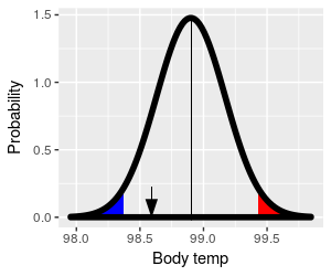
The retention region is centered on the hypothetical population
mean, and it captures 95% of the possible sample means. If you
click on the image you can toggle between using t-values as the
x-axis and using degrees (remember, calculating t is just a
matter of doing a unit conversion to express data units as
standard errors, so we can convert back and forth between the
data units and t-values without changing the shape of the
distribution).
The sample mean 98.7° is the black arrow, and it's within the
retention region - we retain the null, and conclude that the
population mean is 98.6°.
|
The sample mean is a sample-based estimate of the population
mean. A 95% confidence interval centered on the sample mean of
98.7° uses the t-distribution to find limits that capture 95% of
possible sample means. The shaded areas in the tails are the 5%
of the possible sample means that are not in the confidence
interval. Any mean falling within the confidence interval is
considered a possible value for the population parameter.
The hypothetical population mean of 98.6° is shown by the black
arrow. It falls inside of the 95% confidence interval, and we
would conclude that 98.6° is a possible value for the population
mean.
|
With the graph of a t-test on the left set to show units of degrees,
the only difference between the left and right graph is that the left is
centered on the hypothetical value of 98.6°, whereas the graph on the
right is centered on the sample mean of 98.7°. If we center on the
hypothetical population mean, as we do with the t-test, we check if the
sample mean falls inside of the interval around the population mean. If
we center on the sample mean, as we do with a 95% confidence interval,
we check if the hypothetical population mean falls inside of the
interval around the sample mean. In both cases we are using sample
information to infer the properties of the population the sample comes
from.
Why don't we test what we want to know?
Our null hypothesis is that body temperature is equal to 98.6°, but we
didn't calculate the probability that the population mean is equal to
98.6°.
Our sample mean is 98.7°, but we didn't calculate the probability that
the population mean is equal to 98.7°.
Instead, we assumed that the population mean is 98.6°, and calculated
the probability that a random sample from the population would result in
a sample mean that is at least 0.1° away from 98.6°. This might strike
you as being a little more complicated and indirect than just
calculating the probability of the hypothetical value for μ. If so, you
are correct - it is, in fact, more complicated and indirect. But there
are a couple of reasons we calculate the p-value the way we do.
- First, we don't calculate the probability the null hypothesis is
true because we can't. A probability is a number of times an event
occurs divided by the total number of trials. To calculate the
probability that the null hypothesis is true we would have to know how
often when we obtain a sample mean of 98.7° the null is true, and how
often it's false. We can't know this from a single sample of data.
- We also can't calculate the probability that the population mean is
98.7°, for several reasons.
- First, we don't know how often the population mean is equal to
98.7° when the sample mean is equal to 98.7°, and how often it is
not (and can't know from a single sample of data).
- Second, 98.7° is the mean we observed in our data, it is not a
value we hypothesized in advance. If the only reason for
hypothesizing that body temperature for brandy drinkers is 98.7° is
that we got a sample mean equal to that, then our hypothesis test
becomes logically circular.
- Third, if we tried to run a t-test with the population mean, μ,
set to the sample mean, x̄, the t-value would always be (x̄ - μ)/sx̄
= 0, and the p-value would always be 1.
In contrast, we were able to specify a null hypothetical value for μ
exactly, and in advance. This may seem a little odd to you, but it's
actually true that null hypotheses are usually easier to specify,
because we understand random sampling well enough to predict the average
outcome of random sampling exactly. Alternative hypotheses represent
what we expect if our experimental treatments are having an effect, and
if we had the ability to specify alternative hypotheses exactly we would
already know the system so well that hypothesis testing would be
unnecessary. We test null hypotheses because we can.
Another advantage people give for null hypothesis testing is that using
"no difference" as a default conclusion protects us against confirmation
bias, and we need all the help we can get in that regard. For example,
since drinking brandy makes us feel warmer, we might be predisposed to
believe that it raises body temperature. However, we don't test the
hypothesis that drinking brandy makes us warmer - we test the hypothesis
that drinking brandy has no effect on body temperature, and only
conclude that brandy actually makes us warmer if the mean of our
experimental data shows a big enough effect to be statistically
significant. This makes it more difficult for us to favor pet
hypotheses, and makes it easier for us to objectively evaluate the
evidence.
Assumptions of the one-sample t-test
Statistical assumptions are conditions that have to be met in order for
a statistical analysis to work correctly. There are two common sources
of statistical assumptions: A) general assumptions that ensure that data
values that are representative of the population from which they are
selected, and B) specific requirements needed by particular test
procedures for their p-values to be accurate.
General assumptions (A) are common to essentially all statistical
hypothesis tests, regardless of how they obtain their p-values. The two
most common ones are:
- Independence of observations
- Random sampling
Independent observations are needed so that the sample size we report
is equal to the number of distinct measurements of the population we
have. For example, if we selected a single person and measured their
body temperature 20 times we would have less information about human
body temperature than if we measured the temperatures of 20 different
people once each, because repeated measurements of the same person are
not independent. Random sampling is needed to ensure that group means
are unbiased estimates of the population mean.
An example of a specific assumption for a one-sample t-test (B) is:
We assume that the data are normally distributed, because if this is
true the t-distribution is a very accurate model of a sampling
distribution for a continuous variable.
The t-distribution is robust to violations of the
normality assumption - meaning that the p-values are still accurate if
the data are not normally distributed - provided that the non-normality
is not too severe, and that the sample size is large. Large sample sizes
allow us to rely on the central limit theorem (CLT) - remember, the CLT
tells us that the distribution of sample means is bell-shaped for large
sample sizes even when the distribution of data is not, and since the
t-distribution is a bell-shaped sampling distribution it works well for
large sample sizes with any distribution of data. At small sample sizes
a skewed or bimodal distribution of data in the population results in a
sampling distribution that is not bell-shaped, and the t-distribution is
less accurate as a model. Sample sizes of 30 or more are enough to
justify using the t-distribution for all but the most severe violations
of normality.
We will routinely test for normality before we do t-tests. If we
violate normality we will look at the sample size, and if n is 30 or
larger we will go ahead and conduct the t-test in spite of the
non-normality of our data.
Errors in hypothesis testing
When we reject or retain the null, we are making a definite conclusion
based on a probability, which inevitably means that some of our
conclusions will be wrong. We can't eliminate errors from statistical
hypothesis testing, but we can quantify the chances that we are making
one class of mistakes (false positives), and we can take steps to
minimize others (false negatives).
The errors we could make depend on the conclusion we draw.

If we reject the null, we are drawing the right conclusion as
long as the null is false. If the null is true, rejecting it is
a mistake.
We call rejection of a true null a Type I error.
Since we think of a rejected null as a positive result, a Type I
error is also called a false positive. If we
reject the null, the only mistake we could be making is a false
positive, Type I error.
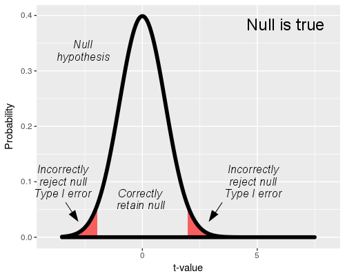
We have a lot of control over our Type I error rate - we
actually get to specify how big we want it to be. The
t-distribution we use in our hypothesis test represents the null
hypothesis, so the "Null is true" graph shows a t-distribution
with the rejection and retention regions identified. When the
null is true, any time a sample mean falls into the rejection
region we would reject the null, which would be a mistake.
The rejection region is set by our choice of alpha level. With
an alpha level of 0.05 and a true null hypothesis, 5% of sample
means will cause us to mistakenly reject the null - thus, the
alpha level is our false positive, Type I error rate. Since we
set alpha to 0.05 for every test we run, it is always the same
regardless of sample size.
|

If we retain the null we reach the correct conclusion if the
null hypothesis is true, but we make a mistake if the null
hypothesis is false.
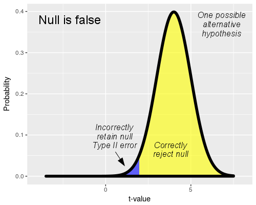
We don't know what the actual population mean is if the null is
false, but to illustrate the mistake we can make when we retain
the null we need to pick one so that a sampling distribution can
be drawn. You'll see that this graph uses a value of t = 4 to
represent the alternative, which is equivalent to a population
mean that is 4 standard errors above the null value (that is,
body temperature of 4 x 0.067 = 0.268 degrees above 98.6°, or μ
= 98.868).
When we do a t-test, the rejection and retention regions are
defined by the null hypothesis, and are the same here as above.
However, if the null is false we are randomly sampling from this
alternative distribution instead of the null distribution above.
The population mean of μ = 98.868 is far enough away from
the null that random samples from this population fall into the
rejection region most of the time - the yellow part of the curve
represents the sample means that cause us to correctly reject
the false null.
However, some of the sample means will be far enough below the
population mean of μ = 98.868 that they fall into the
retention region. When this happens we retain the null in error.
The blue shaded part of the distribution is the portion that
falls into the retention region, and represents the rate at
which we would fail to reject the false null hypothesis.
Failing to reject a null hypothesis that is false is called a
Type II error, which are false negative
errors. The blue shaded area under the curve is the probability
of a Type II error, which is called beta (β).
The yellow portion of the curve also has a name: statistical
power. The yellow part of the curve represents cases
in which we were able to detect an actual difference from the
null value, and the probability of correctly rejecting a false
null is 1-β. We want to be able to detect actual biological
effects when they occur, so rejecting a false null is a good
thing - we want our experiments to give us good statistical
power, like this illustration.
But, there is a problem with calculating Type II error rate and
power.
|
If the null hypothesis is false we don't know what the
actual population mean is (if we knew we wouldn't have to do any
hypothesis testing!). If we picked a different alternative than this one
there would be a different amount of overlap with the retention region,
and the Type II error rate (and thus power) would be different.
Consequently, if we don't know what the actual population mean is then
we can't know what the Type II error rate is either.
So, not only do we not get to specify Type II error rate like
we do Type I error rate, we don't even know what the Type II error rate
is. What we can do, though, is adopt practices in our experiments that
make Type II error rates as low as possible, and thereby increase power,
even if we don't know what the rates actually are.
Minimizing false negatives, increasing
statistical power
So, how do we make β smaller when we don't know its value? In a general
sense, we do this by doing one of two things:
1) make the differences we are trying to detect large, or
2) make the size of the standard error small
 |
Let's look first at how the amount of difference between the
null value and the actual value of the population mean affects
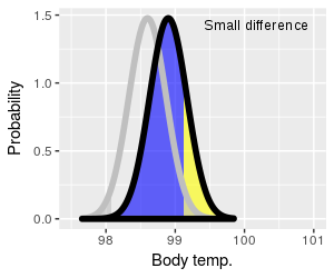
Type II error rate and power. In the graph on the left the
t-distribution for the hypothetical value of 98.6° is shown with
a thick gray line, and the rejection regions are also shaded in
gray. The alternative (which we're assuming now is true) is
shown in black. Instead of using t-values for the x-axis these
graphs use body temperature to make it more clear what is
happening.
You can click on the graph to change it from a small difference
to a large difference. The null curve is in the same place for
both, but the alternative switches from 98.9° to 99.5° as you
switch from small to large difference, respectively.
The blue-shaded region represents false negative (Type II)
errors, and the yellow part of the curve is statistical power.
When the actual population mean is close to the null value
(small difference) most of sample means fall into the retention
region - which means that we can expect most of our experimental
results will give us Type II errors. Power to detect a small
difference is also therefore low (lots of blue, not much
yellow).
When the difference is large, most sample means fall into the
rejection region - most of our experimental results will give us
correct positive test results, so there will be few false
negatives and power will be high (little blue, lots of yellow).
|
|
So, for a given sample size and standard error, the bigger the
difference is that we're trying to detect the greater our power
to detect it will be.
In experiments the way we influence the size of difference we
are trying to detect is in our choice of the size of the
treatment. In our brandy experiment we could increase the
difference by having our subjects drink more brandy - if
drinking brandy affects core body temperature, then drinking
more should cause a bigger change.
However, we don't always have much control over the amount of
difference we are trying to detect - it is often a property of
the system we study, rather than something we get to set. We
also have to be careful about increasing dosages of treatments,
because we don't want to overdose the subjects.
|

|
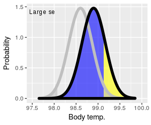
The other way of increasing power is to decrease the size of
the standard error. You can see the effect of reducing standard
error by clicking on the graph to the left, which will switch
between curves with large standard errors (broad curves) and
small ones (narrow curves). Small standard errors increase the
amount of yellow (power), and decrease the amount of blue (Type
II error).
It's important to note that the alternative curves for both
large and small sx̄ have the same mean of 98.9°, so
the increase in power isn't due to the size of difference
getting bigger. Instead, the increase in power is due to the
fact that narrower curves give us more precise estimates of the
actual population mean. This is reflected in the graph as a
smaller retention region, and a larger retention region, when
the standard error is small - the two curves with a small
standard error overlap less, and make it more likely that we'll
sample a mean that falls into the rejection region, and
(correctly) reject the null.
|
As we learned when we encountered standard errors as components of
confidence intervals, there are two ways to reduce the size of a
standard error:
- Decrease the standard deviation (careful measurements, use of
subjects that are similar in size, age, sex, etc.)
- Increase the sample size
Increasing sample size is considered the best way to minimize standard
error size, and is always beneficial to the study. It may not always be
possible to increase sample sizes for practical reasons (i.e. expense,
time constraints, ethical considerations), but bear in mind that using
small sample sizes can end up producing such low statistical power that
the experiment is not worth doing.
Summing up - statistical errors and power
To summarize, here is a table of the errors you can make depending on
whether the null is true or false:
|
Conclusion drawn |
| Reality |
Retain |
Reject |
| Null is true |
No error (1-α) |
Type I error (α)
False positive |
| Null is false |
Type II error (β)
False negative |
No error (power, 1-β) |
Bear in mind - you never know if you made an error, because you never
know if the null is true or false under real-world experimental
conditions. But, if you retain the null the only error you could make is
a Type II error, and if you reject the null you could only have made a
Type I error.
So, what does brandy do to body temperature?
You may know this already (Mythbusters even did an episode on it), but
drinking alcohol does not actually raise your core body temperature.
Alcohol causes the capillaries in your skin to dilate (i.e. increase in
diameter), which allows more blood to flow from your core to the surface
of your body. This makes you feel warm, but by increasing circulation of
blood to your body's surface it actually increases heat loss from your
core. As long as you aren't in a cold environment that's not a big
problem, but for people who already have low core temperatures an
increase in heat loss can cause their temperature to drop further, and
can cause hypothermia and death.
So, believe it or not, Disney cartoons from the 1930's are not a
reliable source of medical information.
Next activity
In this week's activity we will whether our height to stride ratios are
equal to 1.19, which is the value used to estimate heights of suspects
from stride lengths found at crime scenes.


