Introduction - another approach to comparing means
 Consider
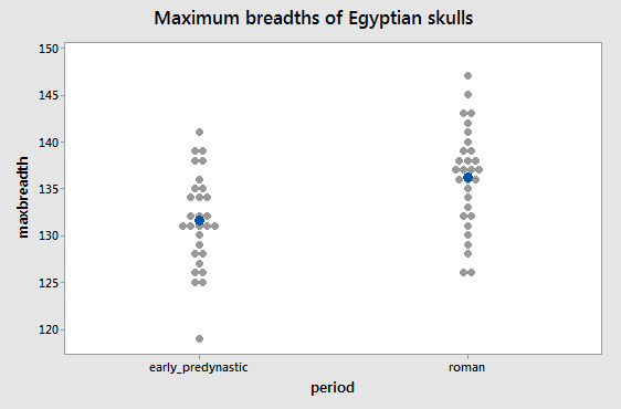
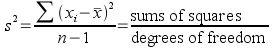
this data of measurements of Egyptian skulls recovered from tombs of the
Early Predynastic period (ca. 4000 BC), and of the Roman period (ca. 150
AD). The variable is the maximum breadth (i.e. width across) the skulls,
and the means are indicated by the blue dots. Individual measurements
are shown as gray dots. You can see that the means are not identical,
but as you should be well aware by now it is possible that the means are
only different due to random sampling variation, and another set of
skulls would show us no difference at all, or a difference just as big
in the opposite direction. To be confident that the periods differed in
their skull breadths we would want to do a statistical null hypothesis
test to see if this difference in sample means is statistically
significant.
Consider
this data of measurements of Egyptian skulls recovered from tombs of the
Early Predynastic period (ca. 4000 BC), and of the Roman period (ca. 150
AD). The variable is the maximum breadth (i.e. width across) the skulls,
and the means are indicated by the blue dots. Individual measurements
are shown as gray dots. You can see that the means are not identical,
but as you should be well aware by now it is possible that the means are
only different due to random sampling variation, and another set of
skulls would show us no difference at all, or a difference just as big
in the opposite direction. To be confident that the periods differed in
their skull breadths we would want to do a statistical null hypothesis
test to see if this difference in sample means is statistically
significant.
The method you know already for making a comparison between two sample means is the two-sample t-test. The two-sample t-test would test the null hypothesis that the population means for both periods are equal, or:
Ho: μearly predynastic = μroman
To complete the test we would calculate an observed t-value, compare it to a t-distribution to obtain a p-value, and then compare the p-value to our alpha level of 0.05. If the p-value is less than 0.05 we would reject the null hypothesis of no difference in favor of the alternative hypothesis that the periods differ in maximum breadth.
The test statistic we use for a two-sample t-test is the observed t-value, which is:
Recall that you can interpret the observed t-statistic as the number of standard errors between the means.
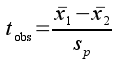
 You
can also think of it as a form of signal to noise ratio.
Signal refers to the information you are trying to detect, and noise
refers to random interference that prevents you from detecting the
signal (think in terms of static in a phone call that prevents you from
hearing the person you're talking to). The images on the left illustrate
the concept using the word "signal" spelled out against random dots of
color in the background. The word is either clearly standing out against
the random noise in the background (bottom), or is barely detectable and
nearly overwhelmed by the noise (top). Weak signals, or noisy
backgrounds, make it difficult to understand the information in your
data.
You
can also think of it as a form of signal to noise ratio.
Signal refers to the information you are trying to detect, and noise
refers to random interference that prevents you from detecting the
signal (think in terms of static in a phone call that prevents you from
hearing the person you're talking to). The images on the left illustrate
the concept using the word "signal" spelled out against random dots of
color in the background. The word is either clearly standing out against
the random noise in the background (bottom), or is barely detectable and
nearly overwhelmed by the noise (top). Weak signals, or noisy
backgrounds, make it difficult to understand the information in your
data.
For the skull data, the signal that you are trying to detect is the difference in means between the periods, and the noise is the random sampling variation that makes it difficult to detect the population-level differences we're interested in. The numerator of the observed t-value measures the signal (difference between group means), and the denominator measures the noise (random sampling variation). The bigger the signal and/or the smaller the noise the bigger the signal to noise ratio will be, and the more likely that your results represent a real difference, and not just random sampling variation.
Another form of signal to noise ratio can be derived from the F
statistic, which we met earlier when we learned to test for homogeneity
of variances between to groups. It's not obvious from what we know so
far how a ratio of two variances could be interpreted as a signal to
noise ratio for the skulls data, but this is done by a procedure called
the Analysis of Variance (ANOVA).
Using variances to compare means
ANOVA is one of the real workhorses of biostatistics. Although the name seems to imply that we're comparing variances between groups, in fact we use ANOVA to test a null hypothesis of no difference between group means. The null hypothesis for an ANOVA that compares two group means can be expressed as:
Ho: μ1 = μ2
just like a two-sample t-test.
To understand how ANOVA works it's helpful to understand that ANOVA begins by treating each skull's maximum breadth as the result of two different processes - a fixed, predictable effect of the period the skull comes from, and random, unpredictable individual variation.
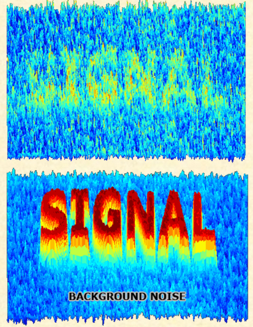
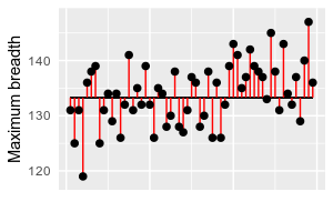
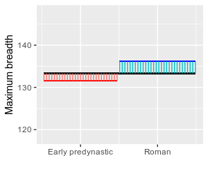
The graph to the left illustrates the skulls data, initially showing the data values for each group color coded with early predynastic in pink and roman in blue. The horizontal black line is the mean of all the data, ignoring group membership, which is called the grand mean. Each point is connected to the grand mean with a vertical red line.
We can think of the lengths of these red lines as partly due to the effect of being either the early predynastic or roman period. If you click on the graph it will change to a graph titled "Variation between group means" that shows the mean for each group as either red horizontal line (early predynastic) or a blue horizontal line (roman). Skulls from the early predynastic period would be expected to be smaller than those from the roman period because the mean for early predynastic is below the grand mean and the mean for roman is above the grand mean. This is the "fixed, predictable effect" of being a skull from one group or the other.
Click again and you'll see a graph titled "Random variation around group means". This shows that the skull measurements are also affected by individual, random differences between skulls. Since we have already accounted for the effect of being from each period using the mean for each period in the previous graph, the vertical lines representing random variation connect to the group mean, rather than the grand mean.
Click again and you'll see both of the processes that determine data values on the same graph (titled "Both sources of variation"). This graph shows that all we are doing is dividing, or partitioning, the data values into an effect of belonging to a group, and an unpredictable, random effect that together determine what the data value is. The predictable effect of belonging to a group is the signal we are trying to detect, and the individual random variation is the noise that obscures the signal.
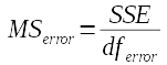
Both of these different contributors to the data values (called sources of variation) are measured in ANOVA using a variance calculation. If you recall, the formula for variance is:
The numerator of a variance calculation is called the sums of squares, which is the part of the calculation that actually measures variability - differences between a group mean (x̄) and individual data values (xi) are squared, and then summed across all of the data values. The denominator is degrees of freedom, which is based on the sample size (n), but with a deduction for any statistics that have to be estimated to calculate the variance - since the mean has to be estimated to calculate the variance, df is sample size minus 1. Dividing by degrees of freedom makes variance an average squared difference between data points and their mean.
To get variances, therefore, we need a sum of squares and a degrees of freedom for each source of variation (between periods - signal, and individual variation within periods - noise) that we can use to calculate the signal to noise ratio we need.
Partitioning variance - sums of squares
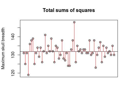
We will start with calculations for sums of
squares, which are raw measures of variation of values around means. The
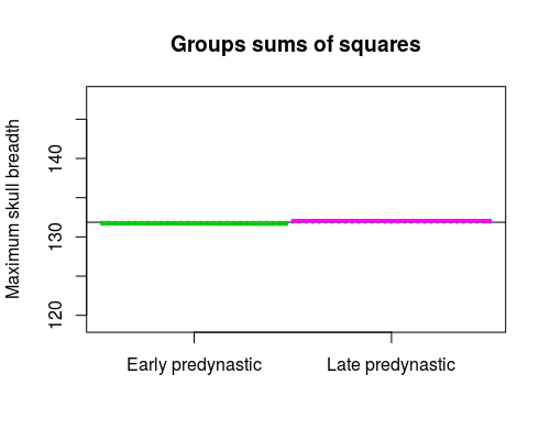
calculations of total sums of squares (SST), groups sums of squares
(SSG), and error sums of squares (SSE) are done like so:
|
Three sources of variation in the skulls data |
|||
|---|---|---|---|
|
|
Total sums of squares |
Groups sums of squares |
Error sums of squares |
|
Graphical illustration: |
 |
 |
 |
|
What it measures: |
Raw measure of variation to be partitioned - individual skulls
varying around the grand mean |
Signal: Measure of the contribution of period means to variation in skull measurements - period means varying around the grand mean |
Noise: Measure of individual, random variation in skulls - individual skulls varying around period means |
|
How it is calculated: |
Subtract the grand mean (x with two bars) from each individual skull's maximum breadth. Each difference is squared, and the squared differences are summed. |
Subtract the grand mean from each period mean (x̄j) and square the differences, once for each data value, and sum them. Since the difference between period mean and grand mean is the same for each skull in a period, this is equivalent to multiplying the squared difference by the number of skulls in the period - thus, the formula is expressed as the differences between group means and the grand mean multiplied by the sample size for the group, nj. |
Subtract the period mean (x̄j) from each individual skull's maximum breadth, square the differences, and sum them. xi,j refers to the i'th data point in period j. |
|
For the skulls data, equal to: |
1841.7 |
304.7 |
1537.0 |
The Total sums of squares (SST) is based on variation around the mean of all the data (called the grand mean), without reference to the period the skull was measured in. This total is not used in our test of differences between periods, but it is a raw measure of all of the variation in the data. To test for differences between periods the total sums of squares is partitioned (that is, divided up) into the two sources of variation we are interested in.
The Period sums of squares (or more generally, the groups sums of squares, SSG) is based on variability of the period means around the grand mean. To the extent that the group means are far apart from one another they will also be far from the grand mean, so variation of group means around the grand mean measures differences between groups.
The Error sums of squares (SSE) is based on variation of individual skulls around the mean of the period it belongs to.
Sums of squares are additive, meaning that SST = SSG + SSE. You can confirm for yourself that 1841.7 = 304.7 + 1537.0
At this point we have partitioned the variation in the data (SST) into a part that is due to predictable differences between the periods (SSG) and a part that is due purely to unpredictable individual random variation (SSE). To complete the analysis we need degrees of freedom to go along with each of these sums of squares.
Partitioning variance - degrees of freedom
The DF term needed for each of our sources of variation are:
- Total: The SST has degrees of freedom just like the formula for variance says it should, n-1. This is the total sample size (n) minus 1. With this data set, this is equal to 59 skulls minus 1 = 58. We refer to this as dftotal.
- Groups: SSG has degrees of freedom of number of groups minus one, or k - 1. There are two groups being compared, so dfgroups is 1.
- Error: SSE has degrees of freedom of sample size minus the number of groups, or n - k. With 59 skulls and 2 groups dferror is 57.
Like sums of squares, degrees of freedom are additive, such that dftotal = dfgroups + dferror, or 58 = 1 + 57.
In ANOVA, variances are called Mean Squares
Now that we have an SS and a DF for each source of variation, we can calculate a variance for each source. In ANOVA we call SS/df the mean squares, but it could just as accurately be called a variance.
The formulas for each MS are:
The total MS for this example is 1841.7/58 = 31.75. This value isn't used in the hypothesis test, so statistical software often does not report it - you'll see that MINITAB doesn't report it in its ANOVA output. |

The groups MS for this example is 304.7/1 = 304.7 |
The error MS for this example is 1537.0/57 = 26.96 |
Sums of squares and degrees of freedom are additive, but mean squares are not (that is, MStotal is not MSgroups+MSerror).
A test statistic - F ratio from MS
We now have all the parts that we need to test for differences between period means - now we just need a test statistic. Since MS are variances, we can use the ratio of MSgroups to MSerror as an F ratio, and test if they are different using an F test, just like we have been doing when we test HOV in a two-sample t-test. Before we do the test, let's consider why this is a test of differences between period means.
Random sampling will always have some effect on the sample means, and thus the variation between groups that is the basis for MSgroups is actually due both to real differences between the period population means (which we'll call fixed effects), and to random sampling variation. Random sampling variation happens because of random variation among individuals, so we can think of MSgroups as actually being:
- MSgroups = Fixed effects of differences between period means + Random, individual variation
If we symbolize the fixed effects of differences between period means with a lower-case Greek gamma, γ, and the individual random variation with e, MSgroups can be represented as γ + e.
MSerror is expected to reflect only individual random variation - that is, it includes the second part of SSG, but not the first part. We can think of MSerror as being only:
- MSerror = Random, individual variation
That is, MSerror is only measuring e.
To get our Fobs test statistic we divide MSgroups by MSerror. Using our symbols, this means that Fobs is measuring:
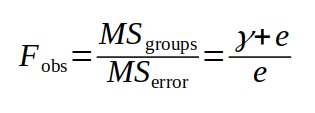
Note that the only difference between what we measure for MSgroups and MSerror is the fixed effect of being in different periods. Under the null hypothesis, there is no actual difference between population means for the two periods, and if this is true, then the fixed effects are equal to 0. If the fixed differences, represented by γ, are actually equal to 0, what would we expect Fobs to be equal to? Click here to see if you're right.
On the other hand, if the null hypothesis is false and there is an actual difference between means, the fixed effects of differences between group means will make MSgroups larger than MSerror, and when we divide MSgroups / MSerror we should get an Fobs value greater than 1.
Since MSgroups is measuring differences between group means (i.e. the signal we're interested in detecting), and MSerror is measuring random variation (i.e. the random noise that makes it difficult to see the differences in mean), this form of the F test statistic is a signal to noise ratio, just like the tobs test statistic was.
In our case, Fobs is equal to 304.7/26.96 = 11.30. With an Fobs greater than 1 there does seem to be more variation between period means than there is within periods. Now we need to know the probability of getting an Fobs of that size by chance when the null hypothesis is true, and the population means are the same between periods.
P-values from F ratios
Once we have a test statistic, Fobs, we need a sampling distribution to tell us the probability of obtaining a value as big or bigger by chance if the null is true, which is the F-distribution.
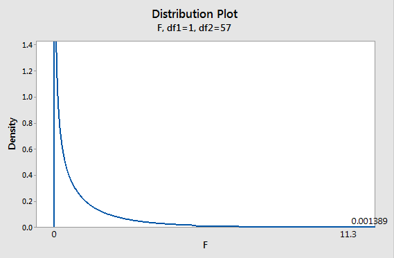 |
Recall from our HOV tests that the F distribution is defined by the df for both of the variances used, and since the F ratio from an ANOVA is always MSgroups/MSerror, the numerator df is the groups df (1 for this analysis), and the denominator df is the error df (57 in this analysis). If there are actual differences between periods we expect MSgroups to be bigger than MSerror, so we're only interested in the upper tail of the F-distribution; that is, ANOVA uses one-tailed F tests. The p-value is the area under the F distribution that falls above Fobs. With our Fobs of 11.3, the p-value is equal to 0.001389. Based on this small p-value, we conclude that the null hypothesis of no difference between periods is rejected - the difference between periods observed is statistically significant. |
The ANOVA table
Now that you understand the basic principles behind an ANOVA, let's look at the traditional method of presenting the results of this test.
An ANOVA is usually presented in a standard format called the ANOVA table. The ANOVA table for the analysis we just completed, above, looks like this:
Source DF Adj SS Adj MS F-Value
P-Value
period 1 304.7 304.73 11.30
0.001
Error 57 1537.0 26.96
Total 58 1841.7
The first row is a set of labels for the columns, which are:
- Source - a label for the source of variation the row is measuring
- DF - degrees of freedom for each source of variation
- (Adj) SS - the sums of squares for each source of variation (don't worry about the "Adj" part - it means "adjusted", but adjustments are only applied for more complicated designs than we will use in this class)
- (Adj) MS - the mean squares for each source of variation (again, ignore the "Adj")
- F-value - the Fobs
- P-value - the p-value for the test of Fobs
Each row is a different source of variation. They are:
- period - the groups source of variation. MINITAB labels the groups by the name of the name of the variable used to identify the groups.
- Error - the random variation between skulls within each group.
- Total - the total variation in the data, which is partitioned into period and error terms
If you look at the contents of the table, you'll see that it's just organizing the various quantities we calculated above. For example:
- The period row gives the groups DF (1), groups SS (304.7), and groups MS (304.73)
- The Error row gives the error DF (57), error SS (1537.0), and error MS (26.96)
- Since Fobs is MSgroups/MSerror, we calculate a single value from two rows in the table. Fobs is a test of differences between period means, so it's placed in the period row.
- The p-value pertains to Fobs, so it is also placed in the period row.
- MStotal isn't used in the test, so it isn't reported. The Total row is primarily presented so that you can verify that total DF is the sum of period and error df, and that total SS is the sum of period and Error SS (this may seem a little silly - we can probably count on MINITAB to be able to add numbers properly - but there are cases in which SS aren't additive, but again these only appear in more complex designs than we're considering).
So, the ANOVA table is a way of organizing a fairly complicated set of calculations into a compact form that's easy to interpret, once you know how it's put together.
ANOVA table
| Source | df | SS | MS | F | p |
|---|---|---|---|---|---|
| Period (groups) | 1 |
304.7 |
304.7 |
11.3 |
0.001 |
| Error | 57 |
1537.0 |
26.96
|
||
| Total | 58 |
1841.7 |
Set the amount of difference between means:
Let's look again at the interpretation of the F value as a signal to noise ratio. This app shows the analysis of the skulls data, but you can use it to to change the amount of difference between the group means so that you can see how the ANOVA table would change as the difference between means increases or decreases. The total sums of squares is held constant by the app, so the focus here is on how the relative amount of variation that's attributable to between-group differences vs. within-group differences translates into either significant or non-significant test results.
If you increase the difference between means you will see that more of the variation in the data is due to differences between periods, which causes the period SS and MS to increase. The period MS is in the numerator of the F value, so as period MS gets larger so does the F-value, which in turn makes the p-value smaller.
If you decrease the difference between the means more of the variation in the data is the within-group, random variation - the groups SS and MS get smaller while the Error SS and MS get larger, which reduces F and causes the p-value to increase. F is thus a measure of the amount of difference between the groups relative to the amount of random variation there is within groups - and, therefore, is a signal to noise ratio.
When the null is true
You have now seen an ANOVA applied to a case with a large, highly
significant difference between means. It is also helpful to think
about what ANOVA results look like when the null hypothesis is true,
and there is no actual difference in population means.
ANOVA table
| Source | df | SS | MS | F | p |
|---|---|---|---|---|---|
| Period | 1 |
304.7 |
304.7 |
11.3 |
0.0014 |
| Error | 57 |
1537.0 |
26.9 |
|
|
| Total | 58 |
1841.7 |
|
|
|
When the null hypothesis is true the only reason sample means for the two periods differ is random chance. If this is true, two random samples from a population with a maximum skull breadth equal to the grand mean of 133.9. The graph on the left shows one set of two random samples (one for each period), with the resulting ANOVA table. The grand mean is indicated with a horizontal gray line labeled "GM", and the mean for each group is a red bar that extends from the grand mean to the group mean for the sample. The p-value will be colored red if it is below 0.05 to help you see when the difference is statistically significant.
If you hit the "Randomize" button you will get a new set of random data for each group. When a pair of random samples results in large differences between the groups the red bars will be big - big differences between groups leads to large SS and MS for Period compared with the unexplained Error variation. This will produce a large F-ratio, and a p-value less than 0.05.
Just like what you saw when you simulated the null hypothesis for a two-sample t-test, you would expect to get a p < 0.05 about 5% of the time, or once every 20 times you hit the "Randomize" button.
Notice that when p is greater than 0.05 the means are relatively close together, compared to the amount of variation around them. Because of this, the Period sums of squares and mean squares are small compared with the error SS and MS, which results in an F ratio (MSPeriod/MSError) that is small. In those approximately 1 in 20 times when p is less than 0.05, the means are farther apart, such that the Period SS and MS are big compared with the error SS and MS, which results in a big F ratio.
Now compare those randomly generated results with a real example - we are still comparing maximum skull breadth for two periods, but now we're comparing early predynastic to late predynastic periods, which are not nearly as different as early predynastic was from the Roman period.
 |
 |
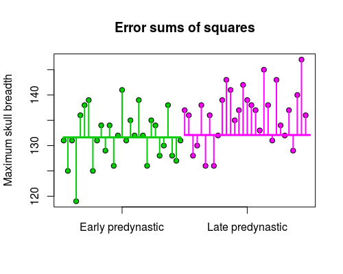 |
You can see that this time the means are very close together, and the groups sums of squares is thus much smaller. Comparatively, there is a lot of random variation compared with this small amount of difference between means. Not surprisingly, when we do all of the calculations and assemble the ANOVA table:
Source DF Adj SS Adj
MS F-Value P-Value
period 1 3.40
3.396 0.14 ...see below...
Error 58 1445.54 24.923
Total 59 1448.93
the F-ratio is much smaller for this comparison: Fobs = 3.396/24.923 = 0.14. We can get the p-value for this comparison by comparing Fobs of 0.14 to an F distribution with 1 numerator and 58 denominator degrees of freedom.
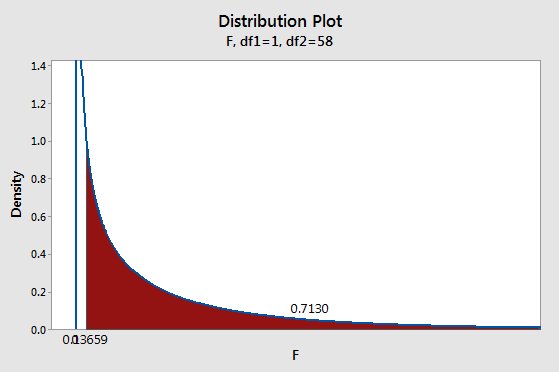 |
The area under the curve from the observed F of 0.14 and above gives us a probability of 0.713. With a p-value over 0.05 we retain the null of no difference between the periods. This amount of difference between means can easily occur by chance when the null is true, so we won't consider the early and late predynastic periods to be different. |
So far all we've done is learn how to do the same analysis using ANOVA that we could have done more simply with a t-test, which might make you wonder why we went to all the trouble.
The reason for learning ANOVA is that the general approach is a much better basis for analyzing complex designs. For this class we'll keep it simple - the only complication we'll consider is the case in which we're comparing more than two groups to one another. We have now used three different periods, but only have tested early predynastic to Roman, and early predynastic to late predynastic periods. We still haven't compared late predynastic to Roman skulls, which we could do by doing one more ANOVA with those two groups, but it's not a good idea - there's a problem with doing multiple comparisons among three or groups two at a time, called the multiple testing problem.
The multiple testing problem
We have now seen data from three different periods (early predynastic, late predynastic, and Roman), but have only compared early predynastic to late predynastic and to Roman periods, but have not compared late predynastic to Roman periods yet. We could make this comparison using a t-test or an ANOVA, but if we do that we would be running a greater risk of making an error in our conclusions that is higher than we expect.
As you know by now, the α-level is the threshold value we compare p against to decide if we have a significant test result or not, and we traditionally use 0.05 as the α-level. But remember, the α-level is also an error rate - it's the probability of rejecting the null hypothesis when it's true. Rejecting a true hypothesis is a mistake, and when we set α to 0.05 we're saying we're willing to make this mistake 5% of the time when we test true null hypotheses. Rejecting a true null is a false positive, which we also call a Type I error, so α is our Type I error rate.
So, each time we test a null hypothesis that's true, we have a probability of making a Type I error of 0.05. If we conduct multiple tests, we take this chance of obtaining a false positive result with each test, and the chance of error accumulates. With three different comparisons, between early predynastic vs. late predynastic, early predynastic vs. roman, and late predynastic vs. roman, our chances of one or more Type I errors is bigger than 0.05, but how big is it?
- If we use the traditional α-level of 0.05, we have a probability of 0.05 of making a mistake with each test
- The probability of not making a mistake on each test is therefore (1-0.05) = 0.95
- The probability of making no mistakes in three tests is just the product of the probability of making no mistakes in a single test - that is, (0.95)(0.95)(0.95), or (0.95)3
- If the probability of no mistakes in three tests is (0.95)3, then the probability of one or more mistakes is 1 - (0.95)3 = 0.14
This means that even though we test each pair of means at α = 0.05, by the time we've finished three tests we actually had a probability of 0.14 of making one or more Type I errors. This inflation of the probability of a false positive with multiple tests is called the multiple testing problem.
ANOVA protects against the multiple testing problem in two ways:
- Unlike t-tests, ANOVA can be compare means between more than two groups. When there are more than two groups to be compared, ANOVA conducts a single initial F test for significant differences among all of the group means, called an omnibus test. The F-test included in the ANOVA table is the omnibus test. The omnibus test indicates if there is reason to think there are differences between two more more of the means being compared, but does not identify which pairs of means are significantly different.
- If and only if the omnibus test is significant, ANOVA can be followed up with a post-hoc procedure to test for differences between pairs of group means so that the groups that are significantly different can be identified. The post-hoc procedure tests for differences between multiple pairs of means in a way that prevents an inflation of Type I error
Let's look at these two methods one at a time.
An omnibus test of differences between three groups using ANOVA
Extending ANOVA to three groups is very simple - the calculations are all the same as for a two group ANOVA, we just have one more group to apply the calculations to.
The null hypothesis with three (or more) groups is like the null hypothesis with two, we just add additional population mean symbols:
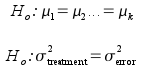
The second way of expressing the null uses variances instead of means (the first variance is labeled "treatment", which is another way of referring to the groups). Since we use an F ratio of mean squares to test for differences among the means, this is also an acceptable way to express the null hypothesis.
|
|
|
This video shows you how an ANOVA on three groups is done. You'll see that there's nothing really different from how we proceeded with only two groups, we just have an additional group mean to use when we calculate SSgroups. Note that the groups SS is illustrated a little differently than before (but the same way as in your book). Now, rather than calculating a difference between a group mean and the grand mean and then multiplying it by the number of data points in the group, the video shows the difference between group mean and grand mean calculated for each data point, which would then be summed together. Adding the same value 30 times is the same as multiplying the value by 30, so it makes no difference which way the groups SS is calculated. |
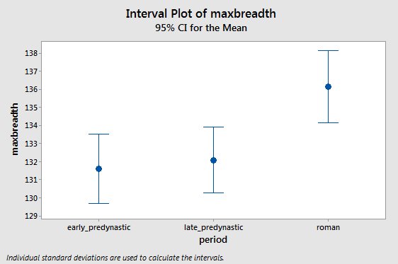 To begin the analysis, it's a good idea to start with a suitable
graph. From this interval plot, it looks like the Roman skulls
have bigger maximum breadths than the other two periods, but the
early and late predynastic periods may not be different from one
another.
To begin the analysis, it's a good idea to start with a suitable
graph. From this interval plot, it looks like the Roman skulls
have bigger maximum breadths than the other two periods, but the
early and late predynastic periods may not be different from one
another. The ANOVA table for these data is here - if you hover over a value in the table a box will appear that explains how it is calculated. Make sure you understand where each entry in the table comes from.
|
SourceThe source of
variation column
|
DFThe degrees of
freedom column
|
SSThe sums of
squares column
|
MSThe mean squares
column
|
FThe Fobs
column
|
PThe p-value column
|
|---|---|---|---|---|---|
|
periodThe row with
the test of differences between periods
|
2DFgroups
= number of groups - 1
|
373.2SSgroups
= sum[group sample size x (group means - grand mean)2]
|
186.6MSgroups
= SSgroups / DFgroups
|
7.13Fobs = MSgroups/MSerror
|
0.001P-value - the
probability of Fobs if the null is true
|
|
ErrorThe row with
individual random variation
|
87DFerror
= sample size - number of groups
|
2275.7SSerror
= sum(data values - group means)2
|
26.16MSerror
= SSerror/DFerror
|
||
|
TotalThe total
variability in the data to be partitioned
|
89DFtotal
= sample size - 1
|
2648.9SStotal
= sum(data values - grand mean)2
|
Based on this table, are there significant differences between the periods? How do you know?
Click here to see if you're right.
At this point, we have three periods, and only one F ratio with one p-value. What can you tell about the differences between periods? Do you know which periods are different from one another?
Click here to see if you're right.
We have now gotten as far as conducting the omnibus test for differences between the periods. There is only one p-value in the table, so we haven't increased our Type I error rate over 0.05, even though we have three group means being compared. That's the good news. The bad news is that we still don't know which periods are different from one another, but we'll fix that problem by conducting a post-hoc procedure called Tukey's MSD.
Post-hoc procedures - Tukey's MSD
Post-hoc procedures are comparisons of pairs of group means conducted after obtaining a significant omnibus test in an ANOVA. They are done in a way that protects against the multiple testing problem, but they are only effective in doing so if they are used following a significant ANOVA.
There are several different post-hoc procedures available in MINITAB, but we will focus in this class on one that seems to work well and is widely used, called the "Tukey Minimum Significant Difference" (or Tukey MSD for short).
Tukey tests look just like t-tests in MINITAB - there is a difference between means, which is divide by a measure of sampling variability to obtain a t-value, and then this test statistic is used to calculate a p-value using a bell-shaped sampling distribution. There are only a couple of differences:
- The measure of sampling variation used is based on the MSerror from the ANOVA instead of using a pooled variance calculation.
- p-values are obtained by comparing Tukey's test statistic to the Studentized range distribution instead of the t-distribution.
The Studentized range distribution is a bell-shaped curve like the t, but its shape is affected by the number of comparisons being conducted. Specifically, the Studentized range distribution requires bigger differences between means in order for them to be considered significant, compared to a t-distribution. The amount of difference needed increases with an increase in the number of groups being compared. If a bigger difference is needed to reject the null, then there will be fewer positive tests, and thus also fewer false positives. Tukey's test thereby protects the α-level, in that the overall probability of a false positive across all the means compared is still 0.05, no matter how many groups are compared.
Let's look at how MINITAB presents ANOVA and Tukey results. After getting a significant omnibus test for differences among periods, we get Tukey results that look like this:
Tukey Simultaneous Tests for Differences of MeansDifference Difference SE of Adjusted
of Levels of Means Difference T-Value P-Value
late_predyna - early_predyn 0.48 1.32 0.36 0.931
roman - early_predyn 4.55 1.33 3.41 0.003
roman - late_predyna 4.07 1.31 3.11 0.007
Each row in this table is a different comparison between means - the comparison used is shown under "Difference of Levels". The first row is a difference between late predynastic and early predynastic periods, and the difference is 0.48 mm. The standard error of the difference is based on the MSerror and the sample sizes of the two groups being compared - the MSerror comes from the ANOVA table and is the same for all comparisons, but there are 29 skulls in the early predynastic period, 31 in late predynastic, and 30 in Roman, so the standard errors are slightly different. The t-values are differences of means divided by standard errors. The p-value is obtained by comparing the t-values to the Studentized Range distribution, which is like a t-distribution that accounts for the number of comparisons being made.
Since Tukey's procedure uses a probability distribution that accounts for the number of tests we're running, the p-value can be interpreted as always - if p is less than 0.05 the difference is significant, and having multiple "adjusted" p-values doesn't inflate our Type I error rate.
Another way that MINITAB uses to illustrate differences between means from a post-hoc procedure is called a compact letter display. For example, if you look at the grouping information output for this test, you'll see:
Grouping Information Using the Tukey Method and 95% Confidenceperiod N Mean Grouping
roman 30 136.167 A
late_predynastic 31 132.097 B
early_predynastic 29 131.621 B
Means that do not share a letter are significantly different.
As the final line in this block of output says, groups that do not share a letter are significantly different. This means that the Roman period is different from both early and late predynastic, but early and late predynastic periods are not different from one another.
Assumptions of ANOVA
ANOVA has similar assumptions to a two-sample t-test - it assumes the data are normally distributed, and that the groups have equal variances. The HOV assumption in ANOVA applies to the amount of variation within each group that is being compared.
Normality
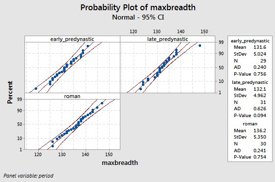
We will test the normality assumption in exactly the same way as we have done with t-tests, using AD tests and normal probability plots. The only difference is that we will often have three or more groups, so we have more normality plots to look at. Normality looks good in all three groups. |
Homogeneity of variances
The fact that we have more than two groups makes it impossible to test HOV using a single F test, so we need a new test. MINITAB offers Levene's test, which is able to test for differences among more than two group variances at a time. If you ever ran an HOV test and forgot to check the box for the "option" of using tests based on normal distribution, you have already seen a Levene's test. Like an F test, the null hypothesis for a Levene's test is that the variances are the same for the three periods, so a p-value over 0.05 means we retain the null and conclude that the variances are equal (that is, we pass the test if p is over 0.05).
Test for Equal Variances: maxbreadth versus
period
Null hypothesis All variances are equal
Alternative hypothesis At least one variance is different
Significance level α = 0.05
95% Bonferroni Confidence Intervals for Standard Deviations
period
N StDev
CI
early_predynastic 29 5.02433 (3.69852,
7.43954)
late_predynastic 31 4.96222 (3.20040,
8.33783)
roman
30 5.35037 (4.10198, 7.58388)
Individual confidence level = 98.3333%
Test
Method Statistic P-Value
Levene
0.23 0.794
You can see that the p-value is well over 0.05, so we pass the HOV test.
Next activity
We will gain experience in using and interpreting ANOVA by comparing the sizes of European cuckoo eggs found in the nests of several species of European songbird.